Week 7 - Causality: DAGs
Due date: Lab 7 - Tuesday, Nov 11, 5pm ET
Why are we learning this?
📖 See what Uber’s data science team says about causal inference: Using Causal Inference to Improve the Uber User Experience
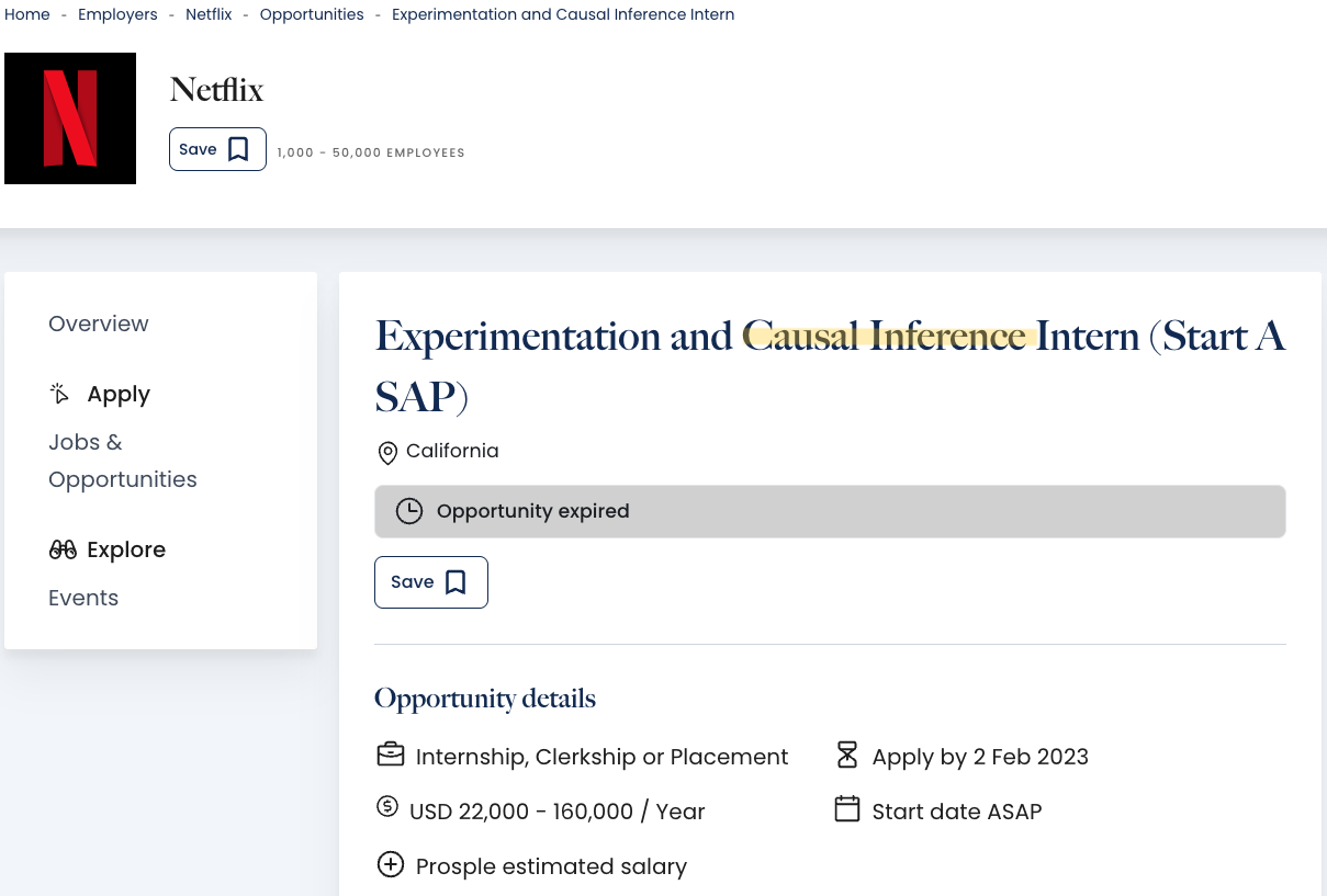
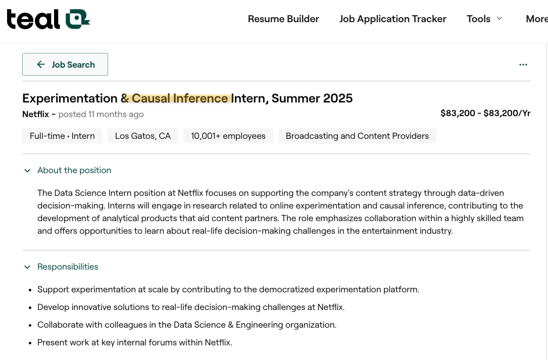
📖 Read about computational Causal Inference at Netflix: Computational Causal Inference at Netflix
📖 Learn about: Machine Learning-Based Causal Inference at Airbnb
📖 See one way banks are Using causal inference for explainability
📖 Find out about the growing “causal revolution” movement in finance
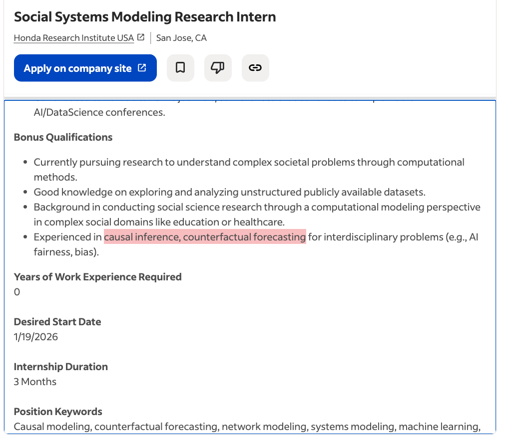
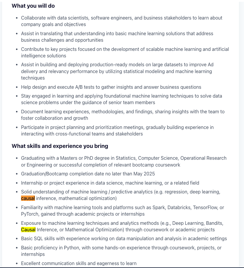
📖 Here’s a recent job posting at Disney and a not so recent job posting at Google and at Netflix
📖 and more:
Advertising.png

Business_research.png

Honda_Research.png
Libra.png

Machine_learning_engineer.png
Netflix_advertising.png

Netflix_intern.png
Netflix_Internship.png

Summer_intern.png
YouTube_Music.png

Prepare
📖 Read Chp 1 in: Statistical Tools for Causal Inference
📖 Read: Demystifying causal inference estimands: ATE, ATT, and ATU or Eight basic rules for causal inference or even A Crash Course in Good and Bad Controls
📖 Read Tutorial on Directed Acyclic Graphs
📖 Read ggdag: An R Package for visualizing and analyzing causal directed acyclic graphs
📖 Read Causal inference & directed acyclic diagrams (DAGs), Chp 7.3-7.4 in (Mostly Clinical) Epidemiology with R
📖 Read Propensity Score Analysis: A Primer and Tutorial Chp 1-4:
📖 Read Marginal Effects Zoo, Inverse Probability Weighting, for treatment evaluation using the marginaleffects package.
📖 Check out this tutorial on causal inference Tutorial 4 - R for Causal Inference.
📖 Review this discussion on the conditions for causal identification S.P.I.C.E of Causal Inference.
Participate
Perform
Study
Short Answer Questions
Instructions: Answer the following questions in 2-3 sentences each.
- Explain the Fundamental Problem of Causal Inference (FPCI).
- What are the three core building blocks of the Rubin Causal Model (RCM)?
- Define “selection bias” in the context of intuitive causal estimators like the “with/without” comparison.
- How does “exchangeability” relate to “identification” in causal inference?
- Describe the key difference between a “fork” (confounder) and a “collider” in a DAG, regarding their implications for statistical correlation between two variables (X and Y) when conditioning on the third variable (Q).
- Why is adjusting for a “collider” problematic when trying to estimate a causal effect?
- What is an “adjustment set” in the context of DAGs, and what is its purpose?
- Briefly explain why “time ordering” variables is a recommended practice when constructing a DAG.
- What is the main goal of Inverse Probability Weighting (IPW) in causal inference?
- Why is bootstrapping often necessary when calculating confidence intervals for propensity-score weighted models?
Short-Answer Answer Key
Explain the Fundamental Problem of Causal Inference (FPCI). The FPCI states that it is impossible to observe both potential outcomes (e.g., what happened if treated and what would have happened if not treated) for the same unit at the same time. This means that for any individual, one of these potential outcomes will always remain unobserved or counterfactual, making direct observation of the unit-level causal effect impossible.
What are the three core building blocks of the Rubin Causal Model (RCM)? The three core building blocks of the Rubin Causal Model are: a treatment allocation rule (deciding who gets treatment), a definition of potential outcomes (outcomes under treatment and control for each unit), and the switching equation (linking observed outcomes to potential outcomes based on treatment allocation).
Define “selection bias” in the context of intuitive causal estimators like the “with/without” comparison. Selection bias is the difference in the untreated potential outcomes between treatment groups ($E[Y_{0i}|D_i=1] - E[Y_{0i}|D_i=0]$). It arises when the treated and untreated groups differ systematically in ways that affect the outcome, even in the absence of treatment, leading to a biased estimate of the true causal effect if not accounted for.
How does “exchangeability” relate to “identification” in causal inference? Exchangeability is an untestable assumption stating that the treated and untreated populations are interchangeable, meaning the joint distribution of potential outcomes is independent of treatment assignment. If exchangeability holds, it often implies identification, which is a mathematical property meaning a causal parameter can be uniquely determined from observable data.
Describe the key difference between a “fork” (confounder) and a “collider” in a DAG, regarding their implications for statistical correlation between two variables (X and Y) when conditioning on the third variable (Q). In a fork (X <- Q -> Y), Q causes both X and Y, leading to a spurious correlation between X and Y. Conditioning on Q blocks this correlation. In contrast, for a collider (X -> Q <- Y), X and Y are not inherently correlated. However, conditioning on the collider Q opens a biasing pathway, inducing a spurious correlation between X and Y.
Why is adjusting for a “collider” problematic when trying to estimate a causal effect? Adjusting for a collider is problematic because it opens a biasing pathway between the two variables that cause the collider, even if they were originally uncorrelated. This can induce a spurious statistical association, leading to a biased estimate of the true causal effect between the exposure and outcome of interest.
What is an “adjustment set” in the context of DAGs, and what is its purpose? An adjustment set is a collection of variables identified from a DAG that, when controlled for (e.g., included in a regression model), can block all backdoor paths between the exposure and outcome. Its purpose is to eliminate confounding bias and allow for the identification of the true causal effect.
Briefly explain why “time ordering” variables is a recommended practice when constructing a DAG. Time ordering variables in a DAG helps clarify causal assumptions because a cause must logically precede its effect. This practice aids in correctly identifying causal relationships and ensures that the diagram accurately reflects the temporal sequence, preventing the inclusion of impossible causal links or cyclic structures.
What is the main goal of Inverse Probability Weighting (IPW) in causal inference? The main goal of IPW is to create a “pseudo-population” where the distributions of observed confounders are balanced between the treated and untreated groups. By re-weighting observations, IPW effectively makes the groups more exchangeable, thereby reducing selection bias and allowing for a more accurate estimation of the average treatment effect.
Why is bootstrapping often necessary when calculating confidence intervals for propensity-score weighted models? Bootstrapping is necessary because the inverse probability weights are not fixed values; they are estimated from the data, introducing an additional source of variability. Standard confidence interval calculations would be too narrow and misleading because they do not account for this dependency and uncertainty in the estimated weights.
Essay Questions
- Discuss the critical role of identification assumptions in causal inference. Choose two specific assumptions (e.g., SUTVA, exchangeability, common support) and explain how their violation would lead to biased causal estimates. Provide a real-world example for each to illustrate the concept.
- Compare and contrast the Average Treatment Effect (ATE) and the Average Treatment Effect on the Treated (ATT). When might a researcher be more interested in one over the other, and what are the implications for the types of data or methods used to estimate each?
- Explain the concept of “selection bias” in detail, including its mathematical definition as presented in the source. Describe how Directed Acyclic Graphs (DAGs) can help identify potential sources of selection bias, specifically focusing on the role of colliders.
- Outline the complete causal inference workflow as presented in the source. For each step, explain its purpose and briefly describe how a researcher would approach it in practice, emphasizing the iterative nature of the process and the importance of expert feedback.
- You are tasked with estimating the causal effect of a new marketing campaign (binary treatment) on customer sales (outcome). Construct a plausible DAG for this scenario, including at least five variables (exposure, outcome, and relevant confounders/mediators/colliders). Based on your DAG, identify a minimal adjustment set and explain why controlling for these variables is necessary to achieve an unbiased estimate.
Back to course schedule ⏎