The Tidymodels Framework

BSMM8740-2-R-2025F [WEEK - 4]

L.L. Odette

Recap of last week

• Last week we looked at several regression methods/models that are useful for predictions.

• However, R packages that implement these methods have different conventions on how they accept data and specify the underlying model.

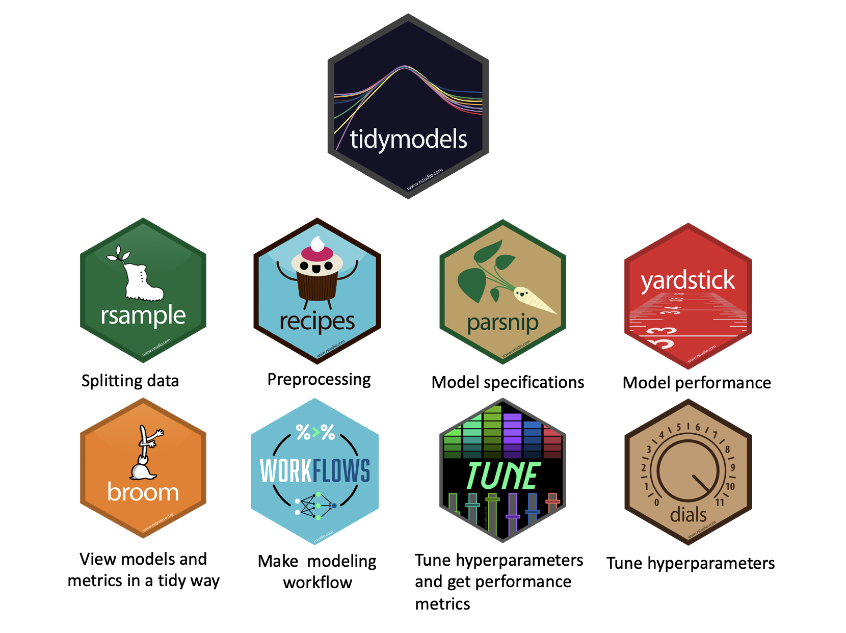
• Today we look at the tidymodels package which will give us a workflow to describe, fit and compare models, using the same approach across methods.

Week 4 Roadmap

• Tidymodels
  • recipes: data pre-processing
  • rsample: data spliting
  • parsnip: model specification
  • tune: model hyperparameters
  • yardstick: model metrics
  • workflows: bundle the above
  • workflowsets: bundle workflows

Tidymodels

Tidymodels

• Tidymodels is a collection of R packages that provides a unified and consistent framework for modeling and machine learning tasks.
• It is built on top of the tidyverse, making it easy to integrate with other tidyverse packages.
• Tidymodels promotes best practices, repeatability, and clear documentation in your data analysis and modeling workflow.

Tidymodels

Key Components of Tidymodels

• Model Building: the parsnip package provides various modeling engines for different algorithms like lm(), glm(), randomForest(), xgboost(), etc.
• Preprocessing: Easy and flexible data preprocessing is provided by the recipes package, allowing for seamless data transformation and feature engineering.

Tidymodels

Key Components of Tidymodels

• Resampling: The rsample package supplies efficient methods for handling data splitting, cross-validation, bootstrapping, and more.
• Metrics: the yardstick package gives a wide range of evaluation metrics to assess model performance and choose the best model.
• Tuning: the tune package facilitates hyperparameter tuning for the tidymodels packages.

Tidymodels

Key Components of Tidymodels

• Workflows: functions in the workflows package can bundle together your pre-processing, modeling, and post-processing requests. The advantages are:
  • You don’t have to keep track of separate objects in your workspace.
  • Both the recipe prepping and model fitting can be executed using a single call to fit().
  • If you have custom tuning parameter settings, these can be defined using a simpler interface when combined with tune.
• Workflowsets: The workflowsets package facilitates multiple workflows - applying different types of models and preprocessing methods on a given data set.

Tidymodels

In base R, the predict function returns results in a format that depends on the model.

By contrast, parsnip and workflows conforms to the following rules:

1. The results are always a tibble.
2. The column names of the tibble are always predictable.
3. There are always as many rows in the result tibble as there are in the input data set, and in the same order.

Tidymodels

Parsnip

Tidymodels: parsnip

We’ve seen how the form of the arguments to linear models in R can be very different¹.

Parsnip is one of the tidymodels packages that provides a standardized interface across models.

We look at how to fit and predict with parsnip in the next few slides, given data that has been preprocessed.

1. e.g. stats::lm takes a formula, while glmnet::glmnet takes separate outcome and co-variate matrices

Fitting with parsnip

For example, we call stats::lm, specifying the model using a formula. By contrast, glmnet::glmnet specify the model with separate outcome and co-variate matrices

The tidymodels permits using both models with a uniform model specification.

Fitting with parsnip

1. Specify the type of model based on its algorithm (e.g., linear regression, random forest, KNN, etc).
2. Specify the engine for fitting the model. Most often this reflects the software package and function that should be used, like lm or glmnet.
3. When required, declare the mode of the model. The mode reflects the type of prediction outcome. For numeric outcomes, the mode is regression; for qualitative outcomes, it is classification.

Fitting with parsnip

With parsnip specifications are built without referencing the data:

• lm
• glmnet

> # basic linear model
> parsnip::linear_reg() %>% 
+   parsnip::set_mode("regression") %>%
+   parsnip::set_engine("lm")

Linear Regression Model Specification (regression)

Computational engine: lm 

> # basic penalized linear model
> parsnip::linear_reg() %>% 
+   parsnip::set_mode("regression") %>%
+   parsnip::set_engine("glmnet")

Linear Regression Model Specification (regression)

Computational engine: glmnet 

Fitting with parsnip

The translate function can be used to see how the parsnip spec is converted to the correct syntax for the underlying package / functions.

• lm
• glmnet

> parsnip::linear_reg() %>% 
+   parsnip::set_engine("lm") %>% 
+   parsnip::set_mode("regression") %>%
+   parsnip::translate()

Linear Regression Model Specification (regression)

Computational engine: lm 

Model fit template:
stats::lm(formula = missing_arg(), data = missing_arg(), weights = missing_arg())

> parsnip::linear_reg(penalty = 1) %>% 
+   parsnip::set_engine("glmnet") %>% 
+   parsnip::set_mode("regression") %>%
+   parsnip::translate()

Linear Regression Model Specification (regression)

Main Arguments:
  penalty = 1

Computational engine: glmnet 

Model fit template:
glmnet::glmnet(x = missing_arg(), y = missing_arg(), weights = missing_arg(), 
    family = "gaussian")

Fitting with parsnip

We can specify the model with either a formula or outcome and model matrix:

> # prep data
> data_split <- rsample::initial_split(modeldata::ames, strata = "Sale_Price")
> ames_train <- rsample::training(data_split)
> ames_test  <- rsample::testing(data_split)
> # spec model
> lm_model <- parsnip::linear_reg() %>%
+   parsnip::set_mode("regression") %>%
+   parsnip::set_engine("lm")
> # fit model
> lm_form_fit <- lm_model %>% 
+   # Recall that Sale_Price has been transformed using log()
+    parsnip::fit(Sale_Price ~ Longitude + Latitude, data = ames_train)
> # fit model with data in (x,y) form
> lm_xy_fit <- 
+   lm_model %>% parsnip::fit_xy(
+     x = ames_train %>% dplyr::select(Longitude, Latitude),
+     y = ames_train %>% dplyr::pull(Sale_Price)
+   )

Fitting with parsnip

Model results can be extracted from the fit object

> lm_form_fit %>% parsnip::extract_fit_engine()

Call:
stats::lm(formula = Sale_Price ~ Longitude + Latitude, data = data)

Coefficients:
(Intercept)    Longitude     Latitude  
 -127338384      -800948      1249366  

> lm_form_fit %>% parsnip::extract_fit_engine() %>% stats::vcov()

              (Intercept)    Longitude      Latitude
(Intercept)  4.771484e+13 364111131502 -323984674156
Longitude    3.641111e+11   3818253249    -156058898
Latitude    -3.239847e+11   -156058898    7359938765

Fitting with parsnip

A list of all parsnip-type models can be found here.

Workflows

Tidymodels: workflows

The workflow data structure collects all the steps of the analysis, including any pre-processing steps, the specification of the model, the model fit itself, as well as potential post-processing activities.

Similar collections of steps are sometimes called pipelines.

Workflows example

Workflows always require a parsnip model object

> # create test/train splits
> ames <- modeldata::ames %>% dplyr::mutate( Sale_Price = log10(Sale_Price) )
> 
> set.seed(502)
> ames_split <- 
+   rsample::initial_split(
+     ames, prop = 0.80, strata = "Sale_Price"
+   )
> ames_train <- rsample::training(ames_split)
> ames_test  <- rsample::testing(ames_split)
> 
> # Create a linear regression model
> lm_model <- parsnip::linear_reg() %>% 
+   parsnip::set_engine("lm") 
> 
> # Create a workflow: adding a parsnip model
> lm_wflow <- 
+   workflows::workflow() %>% 
+   workflows::add_model(lm_model)

Workflows example

If our model is very simple, a standard R formula can be used as a preprocessor:

> # preprocessing not specified; a formula is sufficient
> lm_wflow %<>% 
+   workflows::add_formula(Sale_Price ~ Longitude + Latitude)
> # fit the model ( can be written as fit(lm_wflow, ames_train) )
> lm_fit <- lm_wflow %>% parsnip::fit(ames_train)
> # tidy up the fitted coefficients
> lm_fit %>%
+   # pull the parsnip object
+   workflows::extract_fit_parsnip() %>% 
+   # tidy up the fit results
+   broom::tidy() %>% 
+   # show the first n rows
+   dplyr::slice_head(n=3)

# A tibble: 3 × 5
  term        estimate std.error statistic  p.value
  <chr>          <dbl>     <dbl>     <dbl>    <dbl>
1 (Intercept)  -303.      14.4       -21.0 3.64e-90
2 Longitude      -2.07     0.129     -16.1 1.40e-55
3 Latitude        2.71     0.180      15.0 9.29e-49

Workflows prediction

When using predict(workflow, new_data), no model or preprocessor parameters like those from recipes are re-estimated using the values in new_data.

Take centering and scaling using step_normalize() as an example.

Using this step, the means and standard deviations from the appropriate columns are determined from the training set; new samples at prediction time are standardized using these values from training when predict() is invoked.

Workflows prediction

The fitted workflow can be used to predict outcomes given a new dataset of co-variates. Alternatively, the parsnip::augment function can be used to augment the new data with the prediction and other information about the prediction.

• predict
• augment

> # predict on the fitted workflow
> lm_fit %>% stats::predict(ames_test %>% dplyr::slice(1:3))

# A tibble: 3 × 1
  .pred
  <dbl>
1  5.22
2  5.21
3  5.28

> lm_fit |> 
+   parsnip::augment(new_data = ames_test %>% dplyr::slice(1:3)) |> 
+   dplyr::select( c(starts_with("."), starts_with("MS")) )

# A tibble: 3 × 4
  .pred   .resid MS_SubClass                         MS_Zoning               
  <dbl>    <dbl> <fct>                               <fct>                   
1  5.22 -0.202   One_Story_1946_and_Newer_All_Styles Residential_High_Density
2  5.21  0.174   One_Story_1946_and_Newer_All_Styles Residential_Low_Density 
3  5.28 -0.00629 Two_Story_1946_and_Newer            Residential_Low_Density 

Workflows updating

The model and data pre-processor can be removed or updated:

> # remove the formula and use add_variables instead
> lm_wflow %<>% 
+   workflows::remove_formula() %>% 
+   workflows::add_variables(
+     outcome = Sale_Price, predictors = c(Longitude, Latitude)
+   )

Predictors can be selected using tidyselect selectors, e.g. everything(), ends_with(“tude”), etc.

Workflows use of formulas

We’ve noted that R formulas can specify a good deal of preprocessing, including inline transformations and creating dummy variables, interactions and other column expansions. But some R packages extend the formula in ways that base R functions cannot parse or execute.

When add_formula is executed, since preprocessing is model dependent, workflows attempts to emulate what the underlying model would do whenever possible.

Workflows use of formulas

If a random forest model is fit using the ranger or randomForest packages, the workflow knows predictor columns that are factors should be left as is (not converted to dummy variables).

By contrast, a boosted tree created with the xgboost package requires the user to create dummy variables from factor predictors (since xgboost::xgb.train() will not). A workflow using xgboost will create the indicator columns for this engine. Also note that a different engine for boosted trees, C5.0, does not require dummy variables so none are made by the workflow.

Workflows: special formulas

Some packages have specilized formula specification, i.e. the lme4 package allows random effects per

lme4::lmer(distance ~ Sex + (age | Subject), data = Orthodont)

The effect of this is that each subject will have an estimated intercept and slope parameter for age. Standard R methods can’t properly process this formula.

Workflows: special formulas

In this case The add_variables() specification provides the bare column names, and then the actual formula given to the model is set within add_model():

> multilevel_spec <- parsnip::linear_reg() %>% parsnip::set_engine("lmer")
> 
> multilevel_workflow <- 
+   workflows::workflow() %>% 
+   # Pass the data along as-is: 
+   workflows::add_variables(outcome = distance, predictors = c(Sex, age, Subject)) %>% 
+   workflows::add_model(multilevel_spec, 
+             # This formula is given to the model
+             formula = distance ~ Sex + (age | Subject))

Workflowsets

Tidymodels: workflowsets

Creating multiple workflows at once

The workflowset package creates combinations of workflow components.

A list of preprocessors (e.g., formulas, dplyr selectors, or feature engineering recipe objects) can be combined (i.e. a crossproduct) with a list of model specifications, resulting in a set of workflows.

Tidymodels: workflowsets

Create a set of preprocessors by formula

> # set up a list of formulas
> location <- list(
+   longitude = Sale_Price ~ Longitude,
+   latitude = Sale_Price ~ Latitude,
+   coords = Sale_Price ~ Longitude + Latitude,
+   neighborhood = Sale_Price ~ Neighborhood
+ )
> 
> # create a workflowset
> location_models <- 
+   workflowsets::workflow_set(
+     preproc = location, models = list(lm = lm_model)
+   )

Tidymodels: workflowsets

A workflow set is a nested data structure

> location_models

# A workflow set/tibble: 4 × 4
  wflow_id        info             option    result    
  <chr>           <list>           <list>    <list>    
1 longitude_lm    <tibble [1 × 4]> <opts[0]> <list [0]>
2 latitude_lm     <tibble [1 × 4]> <opts[0]> <list [0]>
3 coords_lm       <tibble [1 × 4]> <opts[0]> <list [0]>
4 neighborhood_lm <tibble [1 × 4]> <opts[0]> <list [0]>

You can extract the elements of the workflowset using tidy::unnest, dplyr::filter, etc. Alternatively the are a number of workflowsets::extract_X functions that will do the job, e.g.

workflowsets::extract_workflow(location_models, id = "coords_lm")

Tidymodels: workflowsets

Create model fits

> # create a new column (fit) by mapping fit 
> # against the data in the info column
> location_models %<>%
+    dplyr::mutate(
+      fit = purrr::map(
+        info
+        , ~ parsnip::fit(.x$workflow[[1]], ames_train)
+       )
+    )
> 
> # view
> location_models$fit[[1]] |> broom::tidy()

# A tibble: 2 × 5
  term        estimate std.error statistic  p.value
  <chr>          <dbl>     <dbl>     <dbl>    <dbl>
1 (Intercept)  -184.      12.6       -14.6 1.97e-46
2 Longitude      -2.02     0.135     -15.0 7.01e-49

Tidymodels: evaluation

Once we’ve settled on a final model there is a convenience function called last_fit() that will fit the model to the entire training set and evaluate it with the testing set. Notice that last_fit() takes a data split as an input, not a dataframe.

> final_lm_res <- tune::last_fit(lm_wflow, ames_split)

• metrics
• predictions

> final_lm_res %>% workflowsets::collect_metrics() 

# A tibble: 2 × 4
  .metric .estimator .estimate .config             
  <chr>   <chr>          <dbl> <chr>               
1 rmse    standard       0.164 Preprocessor1_Model1
2 rsq     standard       0.189 Preprocessor1_Model1

> workflowsets::collect_predictions(final_lm_res) %>% dplyr::slice(1:3)

# A tibble: 3 × 5
  .pred id                .row Sale_Price .config             
  <dbl> <chr>            <int>      <dbl> <chr>               
1  5.22 train/test split     2       5.02 Preprocessor1_Model1
2  5.21 train/test split     4       5.39 Preprocessor1_Model1
3  5.28 train/test split     5       5.28 Preprocessor1_Model1

Yardstick

Tidymodels: yardstick

Performance metrics and inference

Once we have a model, we need to know how well it works. A quantitative approach for estimating effectiveness allows us to understand the model, to compare different models, or to tweak the model to improve performance.

Our focus is on empirical validation; this usually means using data that were not used to create the model as the substrate to measure effectiveness.

Tidymodels: yardstick

When judging model effectiveness, the decision about which metrics to examine can be critical. Choosing the wrong metric can easily result in unintended consequences.

For example, two common metrics for regression models are the root mean squared error (RMSE) and the coefficient of determination (a.k.a. \(R^2\)). The former measures accuracy while the latter measures correlation. These are not necessarily the same thing.

Tidymodels: yardstick

> ames <- dplyr::mutate(modeldata::ames, Sale_Price = log10(Sale_Price))
> 
> set.seed(502)
> ames_split <- rsample::initial_split(ames, prop = 0.80, strata = Sale_Price)
> ames_train <- rsample::training(ames_split)
> ames_test  <- rsample::testing(ames_split)
> 
> ames_rec <- 
+   recipes::recipe(Sale_Price ~ Neighborhood + Gr_Liv_Area + Year_Built + Bldg_Type + 
+            Latitude + Longitude, data = ames_train) %>%
+   recipes::step_log(Gr_Liv_Area, base = 10) %>% 
+   recipes::step_other(Neighborhood, threshold = 0.01) %>% 
+   recipes::step_dummy(
+     recipes::all_nominal_predictors()
+   ) %>% 
+   recipes::step_interact( ~ Gr_Liv_Area:starts_with("Bldg_Type_") ) %>% 
+   recipes::step_ns(Latitude, Longitude, deg_free = 20)
>   
> lm_model <- parsnip::linear_reg() %>% parsnip::set_engine("lm")
> 
> lm_wflow <- 
+   workflows::workflow() %>% 
+   workflows::add_model(lm_model) %>% 
+   workflows::add_recipe(ames_rec)
> 
> lm_fit <- parsnip::fit(lm_wflow, ames_train)

Tidymodels: yardstick

Regression metrics

• prediction
• prediction & obs
• with yardstick

> # fit with new data
> ames_test_res <- 
+   stats::predict(
+     lm_fit
+     , new_data = ames_test %>% dplyr::select(-Sale_Price)
+   )
> ames_test_res

# A tibble: 588 × 1
   .pred
   <dbl>
 1  5.22
 2  5.21
 3  5.28
 4  5.27
 5  5.28
 6  5.28
 7  5.26
 8  5.26
 9  5.26
10  5.24
# ℹ 578 more rows

> # compare predictions with corresponding data
> ames_test_res <- 
+   dplyr::bind_cols(
+     ames_test_res, ames_test %>% dplyr::select(Sale_Price))
> ames_test_res

# A tibble: 588 × 2
   .pred Sale_Price
   <dbl>      <dbl>
 1  5.22       5.02
 2  5.21       5.39
 3  5.28       5.28
 4  5.27       5.28
 5  5.28       5.28
 6  5.28       5.26
 7  5.26       5.73
 8  5.26       5.60
 9  5.26       5.32
10  5.24       4.98
# ℹ 578 more rows

> # there is a standard output format for yardstick functions
> yardstick::rmse(ames_test_res, truth = Sale_Price, estimate = .pred)

# A tibble: 1 × 3
  .metric .estimator .estimate
  <chr>   <chr>          <dbl>
1 rmse    standard       0.164

Tidymodels: yardstick

Regression metrics: multiple metrics at once

> # NOTE: yardstick::metric_set returns a function
> ames_metrics <- 
+   yardstick::metric_set(
+     yardstick::rmse
+     , yardstick::rsq
+     , yardstick::mae
+   )
> 
> ames_metrics(ames_test_res, truth = Sale_Price, estimate = .pred)

# A tibble: 3 × 3
  .metric .estimator .estimate
  <chr>   <chr>          <dbl>
1 rmse    standard       0.164
2 rsq     standard       0.189
3 mae     standard       0.124

Tidymodels: yardstick

Classification metrics: binary class targets

• confusion mat
• accuracy
• mcc
• F-metric

> # compute the confusion matrix: 
> yardstick::conf_mat(
+   modeldata::two_class_example, truth = truth, estimate = predicted
+ )

          Truth
Prediction Class1 Class2
    Class1    227     50
    Class2     31    192

> # compute the accuracy:
> yardstick::accuracy(
+   modeldata::two_class_example, truth, predicted
+ )

# A tibble: 1 × 3
  .metric  .estimator .estimate
  <chr>    <chr>          <dbl>
1 accuracy binary         0.838

> # Matthews correlation coefficient:
> yardstick::mcc(
+   modeldata::two_class_example, truth, predicted
+ )

# A tibble: 1 × 3
  .metric .estimator .estimate
  <chr>   <chr>          <dbl>
1 mcc     binary         0.677

> # F1 metric: (The measure "F" is a combination of precision and recall )  
> yardstick::f_meas(modeldata::two_class_example, truth, predicted)

# A tibble: 1 × 3
  .metric .estimator .estimate
  <chr>   <chr>          <dbl>
1 f_meas  binary         0.849

Tidymodels: yardstick

Classification metrics: binary class targets

> # Combining three classification metrics together
> classification_metrics <- 
+   yardstick::metric_set(
+     yardstick::accuracy
+     , yardstick::mcc
+     , yardstick::f_meas
+   )
> 
> classification_metrics(
+   modeldata::two_class_example
+   , truth = truth
+   , estimate = predicted
+ )

# A tibble: 3 × 3
  .metric  .estimator .estimate
  <chr>    <chr>          <dbl>
1 accuracy binary         0.838
2 mcc      binary         0.677
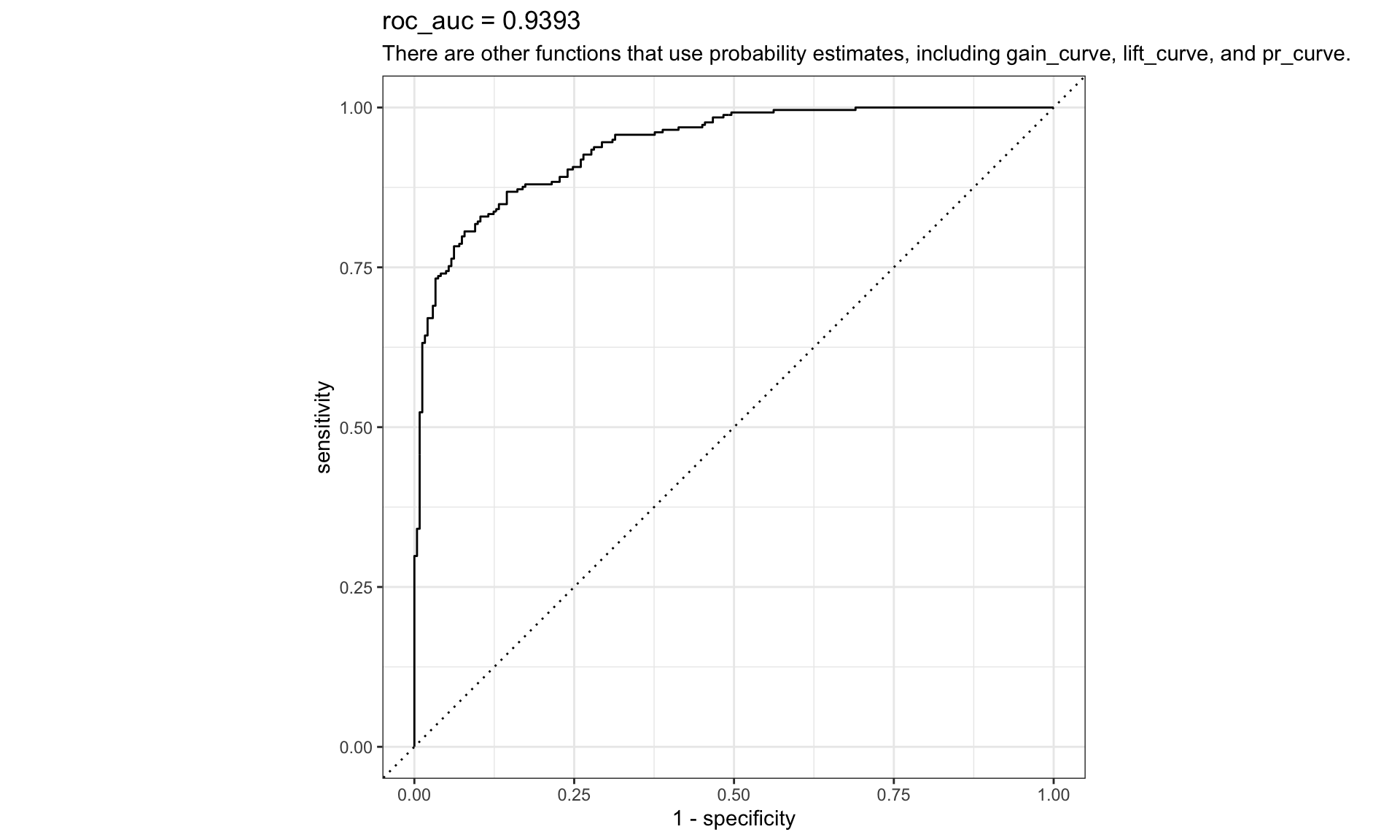
3 f_meas   binary         0.849

Tidymodels: yardstick

Classification metrics: class probabilities

> two_class_curve <- 
+   yardstick::roc_curve(
+     modeldata::two_class_example
+     , truth
+     , Class1
+   )
> 
> parsnip::autoplot(two_class_curve) +
+   labs(
+     title = stringr::str_glue("roc_auc = {round(yardstick::roc_auc(modeldata::two_class_example, truth, Class1)[1,3],4)}") 
+     , subtitle = "There are other functions that use probability estimates, including gain_curve, lift_curve, and pr_curve."
+   )

Sampling / Resampling

Sampling

The primary approach for empirical model validation is to split the existing pool of data into two distinct sets, the training set and the test set.

The training set is used to develop and optimize the model and is usually the majority of the data.

The test set is the remainder of the data, held in reserve to determine the efficacy of the model. It is critical to look at the test set only once; otherwise, it becomes part of the modeling process.

Sampling

The rsample package has tools for making data splits, as follows

> set.seed(501)
> 
> # Save the split information for an 80/20 split of the data
> ames_split <- rsample::initial_split(ames, prop = 0.80)
> ames_split

<Training/Testing/Total>
<2344/586/2930>

The functions training and testing extract the corresponding data.

> ames_train <- rsample::training(ames_split)
> ames_test  <- rsample::testing(ames_split)

Sampling: class imbalance

Simple random sampling is appropriate in many cases but there are exceptions. When there is a dramatic class imbalance in classification problems, one class occurs much less frequently than another. To avoid this, stratified sampling can be used. For regession problems the outcome data can be binned and then stratified sampling will keep the distributions of the outcome similar between the training and test set.

> set.seed(502)
> ames_split <- 
+   rsample::initial_split(ames, prop = 0.80, strata = Sale_Price)
> ames_train <- rsample::training(ames_split)
> ames_test  <- rsample::testing(ames_split)

Sampling: time variables

With time variables, random sampling is not the best choice. The rsample package contains a function called initial_time_split() that is very similar to initial_split() .

The prop argument denotes what proportion of the first part of the data should be used as the training set; the function assumes that the data have been pre-sorted by time in an appropriate order.

Sampling: validation sets

Validation sets are the answer to the question: “How can we tell what is best if we don’t measure performance until the test set?” The validation set is a means to get a rough sense of how well the model performed prior to the test set.

Validation sets are a special case of resampling methods.

> set.seed(52)
> # To put 60% into training, 20% in validation, and 20% in testing:
> ames_val_split <- 
+   rsample::initial_validation_split(ames, prop = c(0.6, 0.2))
> ames_val_split

<Training/Validation/Testing/Total>
<1758/586/586/2930>

The functions validation extracts the corresponding data.

Resampling

While the test set is used for obtaining an unbiased estimate of performance, we usually need to understand the performance of a model or even multiple models before using the test set.

Resampling

Resampling is conducted only on the training set; the test set is not involved.

Resampling: cross-validation

While there are a number of variations, the most common cross-validation method is V-fold cross-validation. The data are randomly partitioned into V sets of roughly equal size (called the folds).

In the example of 3-fold cross validation. In each of 3 iterations, one fold is held out for assessment statistics and the remaining folds are used for modeling.

The final resampling estimate of performance averages each of the V replicates.

In practice, values of V are most often 5 or 10.

Resampling: cv example

> set.seed(1001)
> ames_folds <- rsample::vfold_cv(ames_train, v = 10)
> ames_folds |> dplyr::slice_head(n=5)

# A tibble: 5 × 2
  splits             id    
  <list>             <chr> 
1 <split [2107/235]> Fold01
2 <split [2107/235]> Fold02
3 <split [2108/234]> Fold03
4 <split [2108/234]> Fold04
5 <split [2108/234]> Fold05

The rsample::analysis() and rsample::assessment() functions return the corresponding data frames:

Resampling: repeated cv

The most important variation on cross-validation is repeated V-fold cross-validation. Repeated V-fold cv, reduce noise in the estimate by using more data, i.e. averaging more V statistics.

R repetitions of V-fold cross-validation reduces the standard error variance by a factor of \(1/\sqrt{\text{R}}\).

> rsample::vfold_cv(ames_train, v = 10, repeats = 5) 

#  10-fold cross-validation repeated 5 times 
# A tibble: 50 × 3
   splits             id      id2   
   <list>             <chr>   <chr> 
 1 <split [2107/235]> Repeat1 Fold01
 2 <split [2107/235]> Repeat1 Fold02
 3 <split [2108/234]> Repeat1 Fold03
 4 <split [2108/234]> Repeat1 Fold04
 5 <split [2108/234]> Repeat1 Fold05
 6 <split [2108/234]> Repeat1 Fold06
 7 <split [2108/234]> Repeat1 Fold07
 8 <split [2108/234]> Repeat1 Fold08
 9 <split [2108/234]> Repeat1 Fold09
10 <split [2108/234]> Repeat1 Fold10
# ℹ 40 more rows

Resampling: LOO cv

One variation of cross-validation is leave-one-out (LOO) cross-validation. If there are n training set samples, n models are fit using n−1 rows of the training set.

Each model predicts the single excluded data point. At the end of resampling, the n predictions are pooled to produce a single performance statistic. LOO cv is created using rsample::loo_cv().

Leave-one-out methods are deficient compared to almost any other method. For anything but pathologically small samples, LOO is computationally excessive.

Resampling: MC cv

Another variant of V-fold cross-validation is Monte Carlo cross-validation (MCCV).

The difference between MCCV and regular cross-validation is that, for MCCV, the input proportion of the data is randomly selected each time.

MCCV is performed using rsample::mv_cv().

Resampling: Bootstrapping

Re-sampling: bootstrapping:

A bootstrap sample of the training set is a sample that is the same size as the training set but is drawn with replacement.

When bootstrapping, the assessment set is often called the out-of-bag sample.

> rsample::bootstraps(ames_train, times = 5)

# Bootstrap sampling 
# A tibble: 5 × 2
  splits             id        
  <list>             <chr>     
1 <split [2342/882]> Bootstrap1
2 <split [2342/882]> Bootstrap2
3 <split [2342/858]> Bootstrap3
4 <split [2342/877]> Bootstrap4
5 <split [2342/837]> Bootstrap5

Resampling: Bootstrapping

Each data point has a 63.2% chance of inclusion in the training set at least once.

The assessment set contains all of the training set samples that were not selected for the analysis set (on average, with 36.8% of the training set), and so they can vary in size.

Bootstrap samples produce performance estimates that have very low variance (unlike cross-validation) but have significant pessimistic bias. This means that, if the true accuracy of a model is 90%, the bootstrap would tend to estimate the value to be less than 90%.

bootstrap: draw \(n\) samples with replacement from a dataset of size \(n\)

• chance a given row is not selected in one draw: \(\left(1-\frac{1}{n}\right)\)
• for \(n\) draws, chance the row is not selected: \(\left(1-\frac{1}{n}\right)^n\)
• chance row is included at least once: \(1-\left(1-\frac{1}{n}\right)^n\)

Resampling: time series variables

Re-sampling: resampling time:

When the data have a strong time component, a resampling method needs to support modeling to estimate seasonal and other temporal trends within the data. 

For this type of resampling, the size of the initial analysis and assessment sets are specified and subsequent iterations are shifted in time

Resampling: time variables

Rolling forecast orgin resampling:

Resampling: time variables

Two different configurations of rolling forecast orgin resampling:

• The analysis set can cumulatively grow (as opposed to remaining the same size). After the first initial analysis set, new samples can accrue without discarding the earlier data.
• The resamples need not increment by one. For example, for large data sets, the incremental block could be a week or month instead of a day.

Resampling: time variables

For a year’s worth of data, suppose that six sets of 30-day blocks define the analysis set. For assessment sets of 30 days with a 29-day skip, we can use the rsample package to specify:

> time_slices <- 
+   tibble::tibble(x = 1:365) %>% 
+   rsample::rolling_origin(
+     initial = 6 * 30
+     , assess = 30
+     , skip = 29
+     , cumulative = FALSE
+   )

Resampling: time variables

• analysis
• assessment

> # pull out first and last data points in the analysis dataset
> time_slices$splits %>% 
+   purrr::map_dfr( 
+     .f = ~rsample::analysis(.x) %>% 
+       dplyr::summarize(first = min(.), last = max(.))
+   )

# A tibble: 6 × 2
  first  last
  <int> <int>
1     1   180
2    31   210
3    61   240
4    91   270
5   121   300
6   151   330

> # pull out first and last data points in the assessment dataset
> time_slices$splits %>% 
+   purrr::map_dfr(
+     .f = ~rsample::assessment(.x) %>% 
+       dplyr::summarize(first = min(.), last = max(.))
+   )

# A tibble: 6 × 2
  first  last
  <int> <int>
1   181   210
2   211   240
3   241   270
4   271   300
5   301   330
6   331   360

Tidymodels

Performance evaluation:

1. During resampling, the analysis set is used to preprocess the data, apply the pre-processing to itself, and use these processed data to fit the model.
2. The pre-processing statistics produced by the analysis set are applied to the assessment set. The predictions from the assessment set estimate performance on new data.

This sequence repeats for every resample.

Tidymodels

Performance evaluation:

To reiterate, the process to use resampling is:

1. During resampling, the analysis set is used to preprocess the data, apply the preprocessing to itself, and use these processed data to fit the model.

2. The preprocessing statistics produced by the analysis set are applied to the assessment set. The predictions from the assessment set estimate performance on new data.

Tidymodels

Performance evaluation:

The function tune::fit_resamples is like parsnip::fit with a resamples argument instead of a data argument:

> #
> model_spec %>% tune::fit_resamples(formula,  resamples, ...)
> 
> model_spec %>% tune::fit_resamples(recipe,   resamples, ...)
> 
> workflow   %>% tune::fit_resamples(          resamples, ...)

Tidymodels

Performance evaluation:

Optional arguments are:

• metrics: A metric set of performance statistics to compute. By default, regression models use RMSE and R² while classification models compute the area under the ROC curve and overall accuracy.

• control: A list created by tune::control_resamples() with various options.

Tidymodels

Performance evaluation:

Control arguments are:

• verbose: A logical for printing logging.
• extract: A function for retaining objects from each model iteration (discussed later).
• save_pred: A logical for saving the assessment set predictions.

Tidymodels

Performance evaluation:

Save the predictions in order to visualize the model fit and residuals:

> keep_pred <- 
+   tune::control_resamples(save_pred = TRUE, save_workflow = TRUE)
> 
> set.seed(1003)
> rf_res <- 
+   rf_wflow %>% 
+   tune::fit_resamples(resamples = ames_folds, control = keep_pred)
> rf_res

# Resampling results
# 10-fold cross-validation 
# A tibble: 10 × 5
   splits             id     .metrics         .notes           .predictions      
   <list>             <chr>  <list>           <list>           <list>            
 1 <split [2107/235]> Fold01 <tibble [2 × 4]> <tibble [0 × 3]> <tibble [235 × 4]>
 2 <split [2107/235]> Fold02 <tibble [2 × 4]> <tibble [0 × 3]> <tibble [235 × 4]>
 3 <split [2108/234]> Fold03 <tibble [2 × 4]> <tibble [0 × 3]> <tibble [234 × 4]>
 4 <split [2108/234]> Fold04 <tibble [2 × 4]> <tibble [0 × 3]> <tibble [234 × 4]>
 5 <split [2108/234]> Fold05 <tibble [2 × 4]> <tibble [0 × 3]> <tibble [234 × 4]>
 6 <split [2108/234]> Fold06 <tibble [2 × 4]> <tibble [0 × 3]> <tibble [234 × 4]>
 7 <split [2108/234]> Fold07 <tibble [2 × 4]> <tibble [0 × 3]> <tibble [234 × 4]>
 8 <split [2108/234]> Fold08 <tibble [2 × 4]> <tibble [0 × 3]> <tibble [234 × 4]>
 9 <split [2108/234]> Fold09 <tibble [2 × 4]> <tibble [0 × 3]> <tibble [234 × 4]>
10 <split [2108/234]> Fold10 <tibble [2 × 4]> <tibble [0 × 3]> <tibble [234 × 4]>

Tidymodels

Performance evaluation:

The return value is a tibble similar to the input resamples, along with some extra columns:

• .metrics is a list column of tibbles containing the assessment set performance statistics.
• .notes is list column of tibbles cataloging any warnings/errors generated during resampling.
• .predictions is present when save_pred = TRUE. This list column contains tibbles with the out-of-sample predictions.

Tidymodels

Performance evaluation:

While the list columns may look daunting, they can be easily reconfigured using tidyr or with convenience functions that tidymodels provides. For example, to return the performance metrics in a more usable format:

> rf_res %>% tune::collect_metrics()
> 
> rf_res %>% tune::collect_predictions()
> 
> val_res %>% tune::collect_metrics()

What is collected are the resampling estimates averaged over the individual replicates. To get the metrics for each resample, use the option summarize = FALSE.

Tidymodels: parallelism

The models created during resampling are independent of one another and can be processed in parallel across processors on the same computer.

The code below determines the number of of possible worker processes.

> # The number of physical cores in the hardware:
> parallel::detectCores(logical = FALSE)
> 
> # The number of possible independent processes that can 
> # be simultaneously used:  
> parallel::detectCores(logical = TRUE)

Tidymodels: parallelism

For fit_resamples() and other functions in tune, parallel processing occurs when the user registers a parallel backend package.

These R backend packages define how to execute parallel processing.

Recap

• In this section we have worked with the tidymodels package to build a workflow that facilitates building and evaluating multiple models.

• Combined with the recipes package we now have a complete data modeling framework.