Tidyverse, EDA & git

BSMM8740-2-R-2025F [WEEK - 1]

Dr. L.L. Odette

Welcome to Data Analytic Methods & Algorithms

Announcements

Please go to the course website to review the weekly slides, access the labs, read the syllabus, etc.
My intent is to have assigned lab exercises each week, which will be started during class.
- Lab assignments will be due at 5:00pm sharp on the Sunday following the lecture.
Lab 1 is due Sunday September 14 at 5pm.
My regular office hour will be on Wednesdays from 2:30pm - 3:30pm or via MS Teams as requested. Please email ahead of time.

Expected Course Topics

week	topic
1	The Tidyverse, EDA & Git
2	The Recipes Package
3	Regression Methods
4	The Tidymodels Packages
5	Classification & Clustering Methods
6	Time Series Methods
7	Causality: DAGs
8	Causality: Methods
9	Monte-Carlo Methods
10	Bayesian Methods

Expected Course Topics

analytics	short description	long description
descriptive	what has happened	Calculates trends, averages, medians, standard deviations, etc. Often found in dashboards. Value in providing key statistics.
predictive	what will happen	Finds relationships inside of the data, leading to underlying, generalizable patterns. From patterns, make predictions on unseen data. Value in providing insight on unseen data.
prescriptive	changing what will happen	Uses models created via predictive analytics to recommend optimal actions. Value in finding strategy with the most desirable outcome. Understanding causes of outcomes

Today’s Outline

Introduction to Tidy data & Tidyverse syntax in R.
Introduction to EDA and feature egineering.
Introduction to Git workflows and version control.

Introduction to the Tidyverse

Tidy Data

A dataset is a collection of values, usually either numbers (if quantitative) or strings (if qualitative).

Values are organised in two ways. Every value belongs to a variable and an observation.

A variable contains all values that measure the same underlying attribute (like height, temperature, duration) across units. An observation contains all values measured on the same unit (like a person, or a day, or a business) across attributes.

Tidy Data

Tidy data in practice:

Every column is a variable (aka measurement).
Every row is an observation.
Every cell is a single value.

# A tibble: 6 × 3
  country      year rate             
  <chr>       <dbl> <chr>            
1 Afghanistan  1999 745/19987071     
2 Afghanistan  2000 2666/20595360    
3 Brazil       1999 37737/172006362  
4 Brazil       2000 80488/174504898  
5 China        1999 212258/1272915272
6 China        2000 213766/1280428583

# A tibble: 12 × 4
   country      year type            count
   <chr>       <dbl> <chr>           <dbl>
 1 Afghanistan  1999 cases             745
 2 Afghanistan  1999 population   19987071
 3 Afghanistan  2000 cases            2666
 4 Afghanistan  2000 population   20595360
 5 Brazil       1999 cases           37737
 6 Brazil       1999 population  172006362
 7 Brazil       2000 cases           80488
 8 Brazil       2000 population  174504898
 9 China        1999 cases          212258
10 China        1999 population 1272915272
11 China        2000 cases          213766
12 China        2000 population 1280428583

# A tibble: 6 × 4
  country      year  cases population
  <chr>       <dbl>  <dbl>      <dbl>
1 Afghanistan  1999    745   19987071
2 Afghanistan  2000   2666   20595360
3 Brazil       1999  37737  172006362
4 Brazil       2000  80488  174504898
5 China        1999 212258 1272915272
6 China        2000 213766 1280428583

Tidy Data

We don’t always get data in tidy format
The collection of measurements in an observation is often unique to an organization, and variable names may be non-standard, and
- data may not contain the measurements you need for your business problem

Tidyverse principles

Design for humans
- consistency across packages
- control flow is linear (no loops or jumps)
Reuse existing data structures
- (almost) everything, in and out, is a data frame
Design for functional programming (i.e. the pipe)

Tidyverse packages

Some packages in the tidyverse.

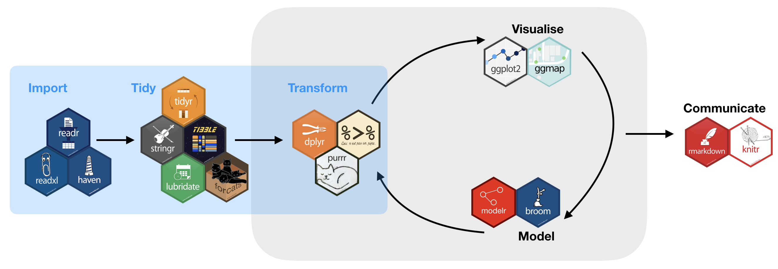
A grammar for data wrangling

The dplyr package gives a grammar for data wrangling, including these 5 verbs for working with data frames.

select(): take a subset of the columns (i.e., features, variables)
filter(): take a subset of the rows (i.e., observations)
mutate(): add or modify existing columns
arrange(): sort the rows
summarize(): aggregate the data across rows (e.g., group it according to some criteria)

A grammar for data wrangling

Each of these functions takes a data frame as its first argument, and returns a data frame.

Being able to combine these verbs with nouns (i.e., data frames) and adverbs (i.e., arguments) creates a flexible and powerful way to wrangle data.

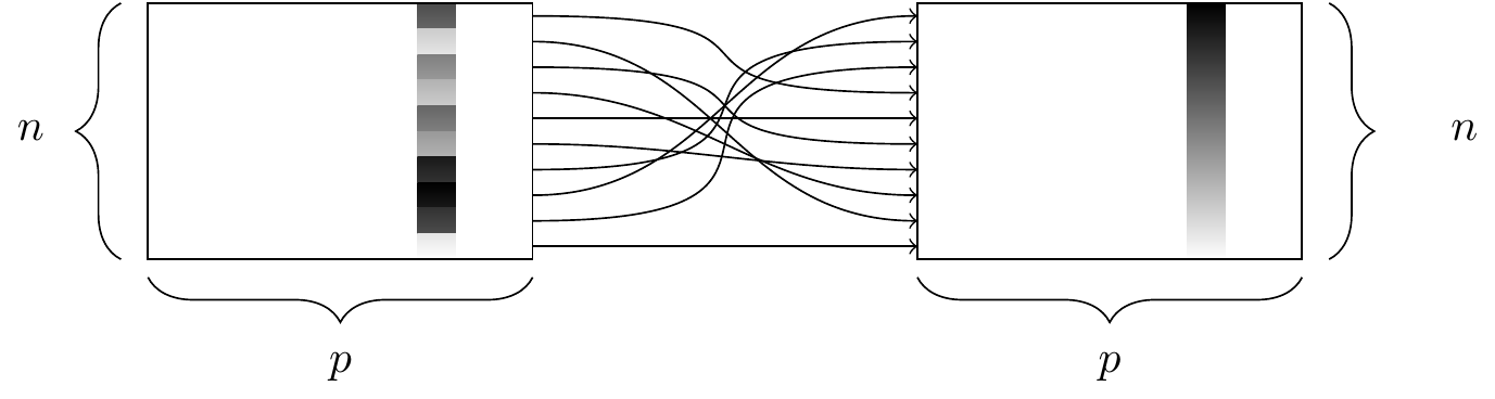
`filter()`

The two simplest of the five verbs are filter() and select(), which return a subset of the rows or columns of a data frame, respectively.

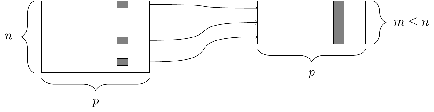
The filter() function. At left, a data frame that contains matching entries in a certain column for only a subset of the rows. At right, the resulting data frame after filtering.

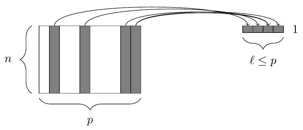
`select()`

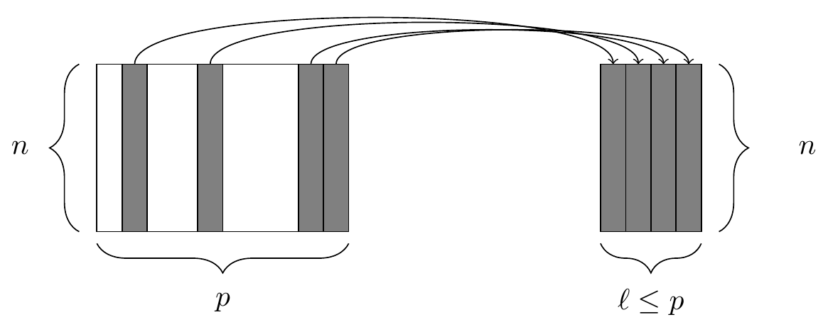
The select() function. At left, a data frame, from which we retrieve only a few of the columns. At right, the resulting data frame after selecting those columns.

Example: data

# A tibble: 28 × 4
   name                start      end        party       
   <chr>               <date>     <date>     <chr>       
 1 John A. Macdonald   1867-07-01 1873-11-05 Conservative
 2 Alexander Mackenzie 1873-11-07 1878-10-08 Liberal     
 3 John A. Macdonald   1878-10-17 1891-06-06 Conservative
 4 John Abbott         1891-06-16 1892-11-24 Conservative
 5 John Thompson       1892-12-05 1894-12-12 Conservative
 6 Mackenzie Bowell    1894-12-21 1896-04-27 Conservative
 7 Charles Tupper      1896-05-01 1896-07-08 Conservative
 8 Wilfrid Laurier     1896-07-11 1911-10-06 Liberal     
 9 Robert Borden       1911-10-10 1920-07-10 Conservative
10 Arthur Meighen      1920-07-10 1921-12-29 Conservative
# ℹ 18 more rows

Example: select

To get just the names and parties of these prime ministers, use select(). The first argument is the data frame, followed by the column names.

dplyr::select(canadian_prime_ministers, name, party)

# A tibble: 28 × 2
   name                party       
   <chr>               <chr>       
 1 John A. Macdonald   Conservative
 2 Alexander Mackenzie Liberal     
 3 John A. Macdonald   Conservative
 4 John Abbott         Conservative
 5 John Thompson       Conservative
 6 Mackenzie Bowell    Conservative
 7 Charles Tupper      Conservative
 8 Wilfrid Laurier     Liberal     
 9 Robert Borden       Conservative
10 Arthur Meighen      Conservative
# ℹ 18 more rows

Example: filter

Similarly, the first argument to filter() is a data frame, and subsequent arguments are logical conditions that are evaluated on any involved columns.

dplyr::filter(canadian_prime_ministers, party == "Conservative")

# A tibble: 11 × 4
   name              start      end        party       
   <chr>             <date>     <date>     <chr>       
 1 John A. Macdonald 1867-07-01 1873-11-05 Conservative
 2 John A. Macdonald 1878-10-17 1891-06-06 Conservative
 3 John Abbott       1891-06-16 1892-11-24 Conservative
 4 John Thompson     1892-12-05 1894-12-12 Conservative
 5 Mackenzie Bowell  1894-12-21 1896-04-27 Conservative
 6 Charles Tupper    1896-05-01 1896-07-08 Conservative
 7 Robert Borden     1911-10-10 1920-07-10 Conservative
 8 Arthur Meighen    1920-07-10 1921-12-29 Conservative
 9 Arthur Meighen    1926-06-29 1926-09-25 Conservative
10 R. B. Bennett     1930-08-07 1935-10-23 Conservative
11 Stephen Harper    2006-02-06 2015-11-04 Conservative

Example: combined operations

Combining the filter() and select() commands enables one to drill down to very specific pieces of information.

dplyr::select(
  dplyr::filter(
    canadian_prime_ministers
    , lubridate::year(start) > 1973 & party == "Liberal"
  )
  , name
)

# A tibble: 5 × 1
  name          
  <chr>         
1 Pierre Trudeau
2 John Turner   
3 Jean Chrétien 
4 Paul Martin   
5 Justin Trudeau

Example: pipe

As written, the filter() operation is nested inside the select() operation.

With the pipe (%>%), we can write the same expression in a more readable syntax.

canadian_prime_ministers %>% 
  dplyr::filter(lubridate::year(start) > 1973 & party == "Liberal") %>%
  dplyr::select(name)

# A tibble: 5 × 1
  name          
  <chr>         
1 Pierre Trudeau
2 John Turner   
3 Jean Chrétien 
4 Paul Martin   
5 Justin Trudeau

`mutate()`

We might want to create, re-define, or rename some of our variables. A graphical illustration of the mutate() operation is shown below

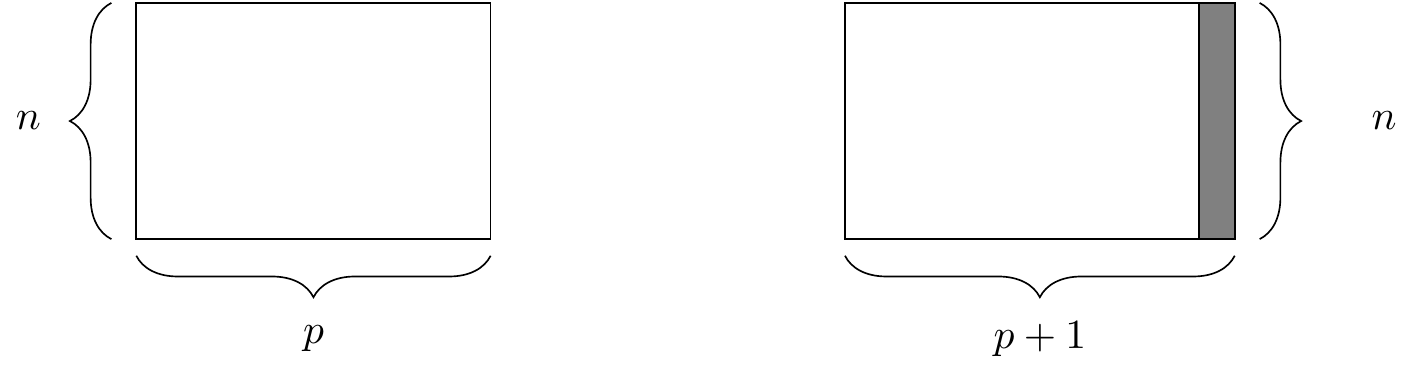
The mutate() function creating a column. At right, the resulting data frame after adding a new column.

Example: mutate, new column

my_prime_ministers <- canadian_prime_ministers %>% 
  dplyr::mutate( 
    term.length = lubridate::interval(start, end) / lubridate::dyears(1) 
  )
my_prime_ministers

# A tibble: 28 × 5
   name                start      end        party        term.length
   <chr>               <date>     <date>     <chr>              <dbl>
 1 John A. Macdonald   1867-07-01 1873-11-05 Conservative       6.35 
 2 Alexander Mackenzie 1873-11-07 1878-10-08 Liberal            4.92 
 3 John A. Macdonald   1878-10-17 1891-06-06 Conservative      12.6  
 4 John Abbott         1891-06-16 1892-11-24 Conservative       1.44 
 5 John Thompson       1892-12-05 1894-12-12 Conservative       2.02 
 6 Mackenzie Bowell    1894-12-21 1896-04-27 Conservative       1.35 
 7 Charles Tupper      1896-05-01 1896-07-08 Conservative       0.186
 8 Wilfrid Laurier     1896-07-11 1911-10-06 Liberal           15.2  
 9 Robert Borden       1911-10-10 1920-07-10 Conservative       8.75 
10 Arthur Meighen      1920-07-10 1921-12-29 Conservative       1.47 
# ℹ 18 more rows

Example: mutate, existing column

The mutate() function can be used to modify existing columns. Below we add a variable containing the year in which each prime minister was elected assuming that every prime minister was elected in the year he took office.

Code

my_prime_ministers %<>% 
  dplyr::mutate(elected = year(start))

# A tibble: 4 × 6
  name                start      end        party        term.length elected
  <chr>               <date>     <date>     <chr>              <dbl>   <dbl>
1 John A. Macdonald   1867-07-01 1873-11-05 Conservative        6.35    1867
2 Alexander Mackenzie 1873-11-07 1878-10-08 Liberal             4.92    1873
3 John A. Macdonald   1878-10-17 1891-06-06 Conservative       12.6     1878
4 John Abbott         1891-06-16 1892-11-24 Conservative        1.44    1891

`rename()`

It is considered bad practice to use a period in names (functions, variables, columns) - we should change the name of the term.length column that we created earlier.

my_prime_ministers %<>% 
  dplyr::rename(term_length = term.length)

# A tibble: 9 × 6
  name                start      end        party        term_length elected
  <chr>               <date>     <date>     <chr>              <dbl>   <dbl>
1 John A. Macdonald   1867-07-01 1873-11-05 Conservative       6.35     1867
2 Alexander Mackenzie 1873-11-07 1878-10-08 Liberal            4.92     1873
3 John A. Macdonald   1878-10-17 1891-06-06 Conservative      12.6      1878
4 John Abbott         1891-06-16 1892-11-24 Conservative       1.44     1891
5 John Thompson       1892-12-05 1894-12-12 Conservative       2.02     1892
6 Mackenzie Bowell    1894-12-21 1896-04-27 Conservative       1.35     1894
7 Charles Tupper      1896-05-01 1896-07-08 Conservative       0.186    1896
8 Wilfrid Laurier     1896-07-11 1911-10-06 Liberal           15.2      1896
9 Robert Borden       1911-10-10 1920-07-10 Conservative       8.75     1911

`arrange()`

The function sort() will sort a vector but not a data frame. The arrange()function sorts a data frame:

The arrange() function. At left, a data frame with an ordinal variable. At right, the resulting data frame after sorting the rows in descending order of that variable.

Example: arrange - sort column

To use arrange you have to specify the data frame, and the column by which you want it to be sorted. You also have to specify the direction in which you want it to be sorted.

my_prime_ministers %>% 
  dplyr::arrange(desc(term_length))

# A tibble: 9 × 6
  name              start      end        party        term_length elected
  <chr>             <date>     <date>     <chr>              <dbl>   <dbl>
1 Wilfrid Laurier   1896-07-11 1911-10-06 Liberal            15.2     1896
2 Mackenzie King    1935-10-23 1948-11-15 Liberal            13.1     1935
3 John A. Macdonald 1878-10-17 1891-06-06 Conservative       12.6     1878
4 Pierre Trudeau    1968-04-20 1979-06-04 Liberal            11.1     1968
5 Jean Chrétien     1993-11-04 2003-12-12 Liberal            10.1     1993
6 Stephen Harper    2006-02-06 2015-11-04 Conservative        9.74    2006
7 Justin Trudeau    2015-11-04 2025-03-14 Liberal             9.36    2015
8 Brian Mulroney    1984-09-17 1993-06-25 PC                  8.77    1984
9 Robert Borden     1911-10-10 1920-07-10 Conservative        8.75    1911

Example, arrange - multiple columns

To break ties, we can further sort by other variables

my_prime_ministers %>% 
  dplyr::arrange(desc(term_length), party, elected)

# A tibble: 28 × 6
   name              start      end        party        term_length elected
   <chr>             <date>     <date>     <chr>              <dbl>   <dbl>
 1 Wilfrid Laurier   1896-07-11 1911-10-06 Liberal            15.2     1896
 2 Mackenzie King    1935-10-23 1948-11-15 Liberal            13.1     1935
 3 John A. Macdonald 1878-10-17 1891-06-06 Conservative       12.6     1878
 4 Pierre Trudeau    1968-04-20 1979-06-04 Liberal            11.1     1968
 5 Jean Chrétien     1993-11-04 2003-12-12 Liberal            10.1     1993
 6 Stephen Harper    2006-02-06 2015-11-04 Conservative        9.74    2006
 7 Justin Trudeau    2015-11-04 2025-03-14 Liberal             9.36    2015
 8 Brian Mulroney    1984-09-17 1993-06-25 PC                  8.77    1984
 9 Robert Borden     1911-10-10 1920-07-10 Conservative        8.75    1911
10 Louis St. Laurent 1948-11-15 1957-06-21 Liberal             8.60    1948
# ℹ 18 more rows

`summarize()` with `group_by()`

The summarize verb is often used with group_by

The summarize() function. At left, a data frame. At right, the resulting data frame after aggregating four of the columns.

Example: summarize - no groups

When used without grouping, summarize() collapses a data frame into a single row.

summarize without groups

my_prime_ministers %>% 
  dplyr::summarize(
    N = n(), 
    first_year = min(year(start)), 
    last_year = max(year(end)), 
    num_libs = sum(party == "Liberal"), 
    years = sum(term_length), 
    avg_term_length = mean(term_length)
  )

# A tibble: 1 × 6
      N first_year last_year num_libs years avg_term_length
  <int>      <dbl>     <dbl>    <int> <dbl>           <dbl>
1    28       1867      2025       13  158.            5.63

Example: pipe - groups

To make comparisons, we can first group then summarize, giving us one summary row for each group.

groups then summarize

my_prime_ministers %>% 
  dplyr::group_by(party) %>% 
  dplyr::summarize(
    N = n(), 
    first_year = min(year(start)), 
    last_year = max(year(end)), 
    num = dplyr::n(), 
    years = sum(term_length), 
    avg_term_length = mean(term_length)
  )

# A tibble: 3 × 7
  party            N first_year last_year   num years avg_term_length
  <chr>        <int>      <dbl>     <dbl> <int> <dbl>           <dbl>
1 Conservative    11       1867      2015    11  49.4            4.49
2 Liberal         13       1873      2025    13  92.4            7.11
3 PC               4       1957      1993     4  15.7            3.93

Example: read_csv & dplyr

# attach package magrittr
require(magrittr)

url <- 
  "https://data.cityofchicago.org/api/views/5neh-572f/rows.csv?accessType=DOWNLOAD&bom=true&format=true"

all_stations <- 
  # Step 1: Read in the data.
  readr::read_csv(url) %>% 
  # Step 2: select columns and rename stationname
  dplyr::select(station = stationname, date, rides) %>% 
  # Step 3: Convert the character date field to a date encoding.
  # Also, put the data in units of 1K rides
  dplyr::mutate(date = lubridate::mdy(date), rides = rides / 1000) %>% 
  # Step 4: Summarize the multiple records using the maximum.
  dplyr::group_by(date, station) %>% 
  dplyr::summarize(rides = max(rides), .groups = "drop")

Magrittr vs native pipe

Topic	Magrittr 2.0.3	Base 4.3.0
Operator	`%>%` `%<>%` `%T>%`	`\|>` (since 4.1.0)
Function call	`1:3 %>% sum()`	`1:3 \|> sum()`
	`1:3 %>% sum`	Needs brackets / parentheses
	1:3 %>% `+`(4)	Some functions are not supported
Placeholder	`.`	`_` (since 4.2.0)

based on a stackoverflow post comparing magrittr pipe to base R pipe.

Use cases for the Magrittr pipe

# functional programming
airlines <- fivethirtyeight::airline_safety %>% 
  # filter rows
  dplyr::filter( stringr::str_detect(airline, 'Air') )

# assignment
airlines %<>% 
  # filter columns and assign result to airlines
  dplyr::select(avail_seat_km_per_week, incidents_85_99, fatalities_85_99)

# side effects
airlines %T>% 
  # report the dimensions
  ( \(x) print(dim(x)) ) %>% 
  # summarize
  dplyr::summarize(avail_seat_km_per_week = sum(avail_seat_km_per_week))

Functions in R

# named function
is_awesome <- function(x = 'Bob') {
  paste(x, 'is awesome!')
}
is_awesome('Keith')

# anonymous function
(function (x) {paste(x, 'is awesome!')})('Keith')

# also anonymous function
(\(x) paste(x, 'is awesome!'))('Keith')

# a function from a formula in the tidyverse
c('Bob','Ted') %>% purrr::map_chr(~paste(.x, 'is awesome!'))

Data Wrangling

The Tidyverse offers a consistent and efficient framework for manipulating, transforming, and cleaning datasets.

Functions like filter(), select(), mutate(), and group_by() allow users to easily subset, reorganize, add, and aggregate data, and the pipe (%>% or |>) enables a sequential and readable flow of operations.

The following examples show a few more of the many useful data wrangling functions in the tidyverse.

Example 1: mutate

mutate
mutate across

openintro::email %>%
  dplyr::select(-from, -sent_email) %>%
  dplyr::mutate(
    day_of_week = lubridate::wday(time)       # new variable: day of week
    , month = lubridate::month(time)          # new variable: month
  ) %>%
  dplyr::select(-time) %>%
  dplyr::mutate(
    cc       = cut(cc, breaks = c(0, 1))      # discretize cc
    , attach = cut(attach, breaks = c(0, 1))  # discretize attach
    , dollar = cut(dollar, breaks = c(0, 1))  # discretize dollar
  ) %>%
  dplyr::mutate(
    inherit = 
      cut(inherit, breaks = c(0, 1, 5, 10, 20))  # discretize inherit, by intervals
    , password = dplyr::ntile(password, 5)       # discretize password, by quintile
  )

iris %>%
  dplyr::mutate(across(c(Sepal.Length, Sepal.Width), round))

iris %>%
  dplyr::mutate(across(c(1, 2), round))

iris %>%
  dplyr::group_by(Species) %>%
  dplyr::summarise(
    across( starts_with("Sepal"), list(mean = mean, sd = sd) )
  )

iris %>%
  dplyr::group_by(Species) %>%
  dplyr::summarise(
    across( starts_with("Sepal"), ~ mean(.x, na.rm = TRUE) )
  )

Example 2: rowwise operations

rowwise operations
using c_across

The verb rowwise creates a special type of grouping where each group consists of a single row.

iris %>%
  dplyr::rowwise() %>%
  dplyr::mutate( 
    mean_length = 
      mean( c(Sepal.Length, Petal.Length) )
    , .before = 1
  ) %>% 
  dplyr::ungroup()

iris %>%
  dplyr::rowwise() %>%
  dplyr::mutate( 
    mean_length = 
      mean(
        dplyr::c_across(c(Sepal.Length:Petal.Width))
      )
    , .before = 1 
  ) %>% 
  dplyr::ungroup()

Example 3: nesting operations

A nested data frame is a data frame where one (or more) columns is a list of data frames.

list columns
group-nesting
mapping

create a list-column of data frames

(df1 <- tibble::tibble(
  g = c(1, 2, 3),
  data = list(
    tibble::tibble(x = 1, y = 2),
    tibble::tibble(x = 4:5, y = 6:7),
    tibble::tibble(x = 10)
  )
) )

# A tibble: 3 × 2
      g data            
  <dbl> <list>          
1     1 <tibble [1 × 2]>
2     2 <tibble [2 × 2]>
3     3 <tibble [1 × 1]>

nest groups by continent, country

(gapminder_nest <- gapminder::gapminder %>% 
  dplyr::mutate(year1950 = year - 1950) %>% 
  dplyr::group_nest(continent, country)
)

# A tibble: 142 × 3
   continent country                                data
   <fct>     <fct>                    <list<tibble[,5]>>
 1 Africa    Algeria                            [12 × 5]
 2 Africa    Angola                             [12 × 5]
 3 Africa    Benin                              [12 × 5]
 4 Africa    Botswana                           [12 × 5]
 5 Africa    Burkina Faso                       [12 × 5]
 6 Africa    Burundi                            [12 × 5]
 7 Africa    Cameroon                           [12 × 5]
 8 Africa    Central African Republic           [12 × 5]
 9 Africa    Chad                               [12 × 5]
10 Africa    Comoros                            [12 × 5]
# ℹ 132 more rows

Fit a linear model for each country:

(gapminder_model <- gapminder_nest %>% 
  dplyr::mutate(
    model = 
      purrr::map(
        data
        , ~lm(lifeExp ~ year1950, data = .))
  ))

# A tibble: 142 × 4
   continent country                                data model 
   <fct>     <fct>                    <list<tibble[,5]>> <list>
 1 Africa    Algeria                            [12 × 5] <lm>  
 2 Africa    Angola                             [12 × 5] <lm>  
 3 Africa    Benin                              [12 × 5] <lm>  
 4 Africa    Botswana                           [12 × 5] <lm>  
 5 Africa    Burkina Faso                       [12 × 5] <lm>  
 6 Africa    Burundi                            [12 × 5] <lm>  
 7 Africa    Cameroon                           [12 × 5] <lm>  
 8 Africa    Central African Republic           [12 × 5] <lm>  
 9 Africa    Chad                               [12 × 5] <lm>  
10 Africa    Comoros                            [12 × 5] <lm>  
# ℹ 132 more rows

Example 4: stringr string functions

Main verbs, each taking a pattern as input

stringr::str_{X}
stringr::str_glue

x <- c("why", "video", "cross", "extra", "deal", "authority")

stringr::str_detect(x, "[aeiou]")       # identifies any matches
stringr::str_count(x, "[aeiou]")        # counts number of patterns
stringr::str_subset(x, "[aeiou]")       # extracts matching components
stringr::str_extract(x, "[aeiou]")      # extracts text of the match
stringr::str_replace(x, "[aeiou]", "?") # replaces matches with new text:
stringr::str_split(x, ",")              # splits up a string

mtcars %>% 
  tibble::rownames_to_column(var = "car") %>% 
  tibble::as_tibble() %T>% 
  (\(x) print(names(x)) ) %>% 
  dplyr::mutate(
    note = stringr::str_glue("The {car} has {cyl} cylinders")) %>% 
  dplyr::slice_head(n=3)

cheat sheet

Example 5: Database functions

Create DB
Extract SQL
Execute Query

# directly like a tibble
db <- 
  dbplyr::memdb_frame(
    x = runif(100)
    , y = runif(100)
    , .name = 'test_tbl'
  )

# using an existing table
mtcars_db <- dbplyr::tbl_memdb(mtcars)

Generate SQL without executing

mtcars_db %>% 
  dplyr::group_by(cyl) %>% 
  dplyr::summarise(n = n()) %>% 
  dplyr::show_query()

<SQL>
SELECT `cyl`, COUNT(*) AS `n`
FROM `mtcars`
GROUP BY `cyl`

Execute Query on DB

mtcars_db %>% 
  dplyr::group_by(cyl) %>% 
  dplyr::summarise(n = n()) %>% 
  dplyr::collapse()

# Source:   SQL [?? x 2]
# Database: sqlite 3.50.1 [:memory:]
    cyl     n
  <dbl> <int>
1     4    11
2     6     7
3     8    14

Extract SQL Example

Execute Query on DB

con <- DBI::dbConnect(RSQLite::SQLite(), dbname = ":memory:")
dplyr::copy_to(con, tibble::tibble(x = 1:100), "temp_table")

dplyr::tbl(con, "temp_table") %>% 
  dplyr::count(
    x_bin = cut(
      x
      , breaks = c(0, 33, 66, 100)
      , labels = c("low", "mid", "high")
    )
  ) %>% 
  dplyr::show_query()

<SQL>
SELECT `x_bin`, COUNT(*) AS `n`
FROM (
  SELECT
    `temp_table`.*,
    CASE
WHEN (`x` <= 0.0) THEN NULL
WHEN (`x` <= 33.0) THEN 'low'
WHEN (`x` <= 66.0) THEN 'mid'
WHEN (`x` <= 100.0) THEN 'high'
WHEN (`x` > 100.0) THEN NULL
END AS `x_bin`
  FROM `temp_table`
) AS `q01`
GROUP BY `x_bin`

Pivoting

longer
wider

When some of the column names are not names of variables, but values of a variable.

# A tibble: 3 × 3
  country     `1999` `2000`
  <chr>        <dbl>  <dbl>
1 Afghanistan    745   2666
2 Brazil       37737  80488
3 China       212258 213766

Pivot longer

tidyr::table4a %>% 
  pivot_longer(
    c(`1999`, `2000`)
    , names_to = "year", values_to = "cases")

# A tibble: 6 × 3
  country     year   cases
  <chr>       <chr>  <dbl>
1 Afghanistan 1999     745
2 Afghanistan 2000    2666
3 Brazil      1999   37737
4 Brazil      2000   80488
5 China       1999  212258
6 China       2000  213766

When an observation is scattered across multiple rows.

# A tibble: 12 × 4
   country      year type            count
   <chr>       <dbl> <chr>           <dbl>
 1 Afghanistan  1999 cases             745
 2 Afghanistan  1999 population   19987071
 3 Afghanistan  2000 cases            2666
 4 Afghanistan  2000 population   20595360
 5 Brazil       1999 cases           37737
 6 Brazil       1999 population  172006362
 7 Brazil       2000 cases           80488
 8 Brazil       2000 population  174504898
 9 China        1999 cases          212258
10 China        1999 population 1272915272
11 China        2000 cases          213766
12 China        2000 population 1280428583

Pivot wider

tidyr::table2 %>%
    pivot_wider(
      names_from = type
      , values_from = count)

# A tibble: 6 × 4
  country      year  cases population
  <chr>       <dbl>  <dbl>      <dbl>
1 Afghanistan  1999    745   19987071
2 Afghanistan  2000   2666   20595360
3 Brazil       1999  37737  172006362
4 Brazil       2000  80488  174504898
5 China        1999 212258 1272915272
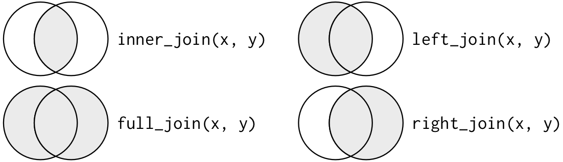
6 China        2000 213766 1280428583

Relational data¹

We can join related tables in a variety of ways:

Relational data

example tables

x <- tibble::tibble(key=1:3, val_x= paste0('x',1:3))
y <- tibble::tibble(key=c(1,2,4), val_y= paste0('y',1:3))

inner join
full join
left join
right join

x %>% dplyr::inner_join(y, by = "key")

# A tibble: 2 × 3
    key val_x val_y
  <dbl> <chr> <chr>
1     1 x1    y1   
2     2 x2    y2

x %>% dplyr::full_join(y, by = "key")

# A tibble: 4 × 3
    key val_x val_y
  <dbl> <chr> <chr>
1     1 x1    y1   
2     2 x2    y2   
3     3 x3    <NA> 
4     4 <NA>  y3

x %>% dplyr::left_join(y, by = "key")

# A tibble: 3 × 3
    key val_x val_y
  <dbl> <chr> <chr>
1     1 x1    y1   
2     2 x2    y2   
3     3 x3    <NA>

x %>% dplyr::right_join(y, by = "key")

# A tibble: 3 × 3
    key val_x val_y
  <dbl> <chr> <chr>
1     1 x1    y1   
2     2 x2    y2   
3     4 <NA>  y3

Relational data

Keys used in the join:

default (e.g. by=NULL): all variables that appear in both tables
a character vector (e.g. by = “x”) uses only the common variables named
a named character vector (e.g. by = c(“a” = “b”)) matches variable ‘a’ in x with variable ‘b’ in y.

Relational data

Filtering Joins:

semi_join(x, y) keeps all observations in x that have a match in y ( i.e. no NAs).
anti_join(x, y) drops all observations in x that have a match in y.

Set operations

When tidy dataset x and y have the same variables, set operations work as expected:

intersect(x, y): return only observations in both x and y.
union(x, y): return unique observations in x and y.
setdiff(x, y): return observations in x, but not in y.

Tidying

tidyr::table3 %>% 
  tidyr::separate_wider_delim(
    cols = rate
    , delim = "/"
    , names = c("cases", "population") 
)

# A tibble: 6 × 4
  country      year cases  population
  <chr>       <dbl> <chr>  <chr>     
1 Afghanistan  1999 745    19987071  
2 Afghanistan  2000 2666   20595360  
3 Brazil       1999 37737  172006362 
4 Brazil       2000 80488  174504898 
5 China        1999 212258 1272915272
6 China        2000 213766 1280428583

Exploratory Data Analysis (EDA)

Exploratory data analysis is the process of understanding a new dataset by looking at the data, constructing graphs, tables, and models. We want to understand three aspects:

each individual variable by itself;
each individual variable in the context of other, relevant, variables; and
the data that are not there.

Exploratory Data Analysis (EDA)

We will perform two broad categories of EDA:

Descriptive Statistics, which includes mean, median, mode, inter-quartile range, and so on.
Graphical Methods, which includes histogram, density estimation, box plots, and so on.

EDA: view all data

Our first dataset is a sample of categorical variables from the General Social Survey, a long-running US survey conducted by the independent research organization NORC at the University of Chicago.

Code

dat <- forcats::gss_cat
dat %>% utils::head()

# A tibble: 6 × 9
   year marital         age race  rincome        partyid     relig denom tvhours
  <int> <fct>         <int> <fct> <fct>          <fct>       <fct> <fct>   <int>
1  2000 Never married    26 White $8000 to 9999  Ind,near r… Prot… Sout…      12
2  2000 Divorced         48 White $8000 to 9999  Not str re… Prot… Bapt…      NA
3  2000 Widowed          67 White Not applicable Independent Prot… No d…       2
4  2000 Never married    39 White Not applicable Ind,near r… Orth… Not …       4
5  2000 Divorced         25 White Not applicable Not str de… None  Not …       1
6  2000 Married          25 White $20000 - 24999 Strong dem… Prot… Sout…      NA

EDA: view all columns

Use dplyr::glimpse() to see every column in a data.frame

dat %>% dplyr::slice_head(n=10) %>% dplyr::glimpse()

Rows: 10
Columns: 9
$ year    <int> 2000, 2000, 2000, 2000, 2000, 2000, 2000, 2000, 2000, 2000
$ marital <fct> Never married, Divorced, Widowed, Never married, Divorced, Mar…
$ age     <int> 26, 48, 67, 39, 25, 25, 36, 44, 44, 47
$ race    <fct> White, White, White, White, White, White, White, White, White,…
$ rincome <fct> $8000 to 9999, $8000 to 9999, Not applicable, Not applicable, …
$ partyid <fct> "Ind,near rep", "Not str republican", "Independent", "Ind,near…
$ relig   <fct> Protestant, Protestant, Protestant, Orthodox-christian, None, …
$ denom   <fct> "Southern baptist", "Baptist-dk which", "No denomination", "No…
$ tvhours <int> 12, NA, 2, 4, 1, NA, 3, NA, 0, 3

EDA: view some rows

Use dplyr::slice_sample() to see a random selection of rows in a data.frame

dat %>% dplyr::slice_sample(n=10)

# A tibble: 10 × 9
    year marital         age race  rincome        partyid    relig denom tvhours
   <int> <fct>         <int> <fct> <fct>          <fct>      <fct> <fct>   <int>
 1  2010 Married          46 White $25000 or more Independe… Cath… Not …       2
 2  2014 Widowed          79 Black Not applicable Strong de… Prot… Am b…       2
 3  2006 Divorced         63 White $25000 or more Independe… Prot… Unit…      NA
 4  2014 Married          54 White $25000 or more Ind,near … None  Not …      NA
 5  2002 Never married    49 Black Refused        Not str d… Prot… Am b…       3
 6  2000 Divorced         66 White Not applicable Independe… Prot… No d…       8
 7  2002 Married          53 White $25000 or more Not str r… Prot… Other      NA
 8  2012 Divorced         63 White Not applicable Ind,near … Cath… Not …      NA
 9  2014 Married          88 White Not applicable Independe… Chri… No d…       3
10  2012 Widowed          86 White Not applicable Independe… Prot… Luth…       4

There are many dplyr::slice_{X} variants, along with dplyr::filter

bad data $\rightarrow$ bad results

EDA: descriptive statistics

The base R function summary() can be used for key summary statistics of the data.

dat %>% summary()

      year               marital           age                    race      
 Min.   :2000   No answer    :   17   Min.   :18.00   Other         : 1959  
 1st Qu.:2002   Never married: 5416   1st Qu.:33.00   Black         : 3129  
 Median :2006   Separated    :  743   Median :46.00   White         :16395  
 Mean   :2007   Divorced     : 3383   Mean   :47.18   Not applicable:    0  
 3rd Qu.:2010   Widowed      : 1807   3rd Qu.:59.00                         
 Max.   :2014   Married      :10117   Max.   :89.00                         
                                      NA's   :76                            
           rincome                   partyid            relig      
 $25000 or more:7363   Independent       :4119   Protestant:10846  
 Not applicable:7043   Not str democrat  :3690   Catholic  : 5124  
 $20000 - 24999:1283   Strong democrat   :3490   None      : 3523  
 $10000 - 14999:1168   Not str republican:3032   Christian :  689  
 $15000 - 19999:1048   Ind,near dem      :2499   Jewish    :  388  
 Refused       : 975   Strong republican :2314   Other     :  224  
 (Other)       :2603   (Other)           :2339   (Other)   :  689  
              denom          tvhours      
 Not applicable  :10072   Min.   : 0.000  
 Other           : 2534   1st Qu.: 1.000  
 No denomination : 1683   Median : 2.000  
 Southern baptist: 1536   Mean   : 2.981  
 Baptist-dk which: 1457   3rd Qu.: 4.000  
 United methodist: 1067   Max.   :24.000  
 (Other)         : 3134   NA's   :10146

EDA: packages for EDA

The function skimr::skim() gives an enhanced version of base R’s summary() .
Other packages, such as DataExplorer:: rely more on graphical presentation.

`skimr::skim()`

numeric variables
factor variables

skim_dat[["numeric"]]

Variable type: numeric

skim_variable	n_missing	complete_rate	mean	sd	p0	p25	p50	p75	p100	hist
year	0	1.00	2006.50	4.45	2000	2002	2006	2010	2014	▇▃▇▂▆
age	76	1.00	47.18	17.29	18	33	46	59	89	▇▇▇▅▂
tvhours	10146	0.53	2.98	2.59	0	1	2	4	24	▇▂▁▁▁

skim_dat[["factor"]]

Variable type: factor

skim_variable	complete_rate	ordered	n_unique	top_counts
marital	1	FALSE	6	Mar: 10117, Nev: 5416, Div: 3383, Wid: 1807
race	1	FALSE	3	Whi: 16395, Bla: 3129, Oth: 1959, Not: 0
rincome	1	FALSE	16	$25: 7363, Not: 7043, $20: 1283, $10: 1168
partyid	1	FALSE	10	Ind: 4119, Not: 3690, Str: 3490, Not: 3032
relig	1	FALSE	15	Pro: 10846, Cat: 5124, Non: 3523, Chr: 689
denom	1	FALSE	30	Not: 10072, Oth: 2534, No : 1683, Sou: 1536

EDA: factor variable counts

Most of the columns here are factors (categories). Use these to count the number of observations per category.

forecats::fct_count
dplyr::count
table()

forcats::fct_count(dat$relig) %>% dplyr::arrange(desc(n))

# A tibble: 16 × 2
   f                           n
   <fct>                   <int>
 1 Protestant              10846
 2 Catholic                 5124
 3 None                     3523
 4 Christian                 689
 5 Jewish                    388
 6 Other                     224
 7 Buddhism                  147
 8 Inter-nondenominational   109
 9 Moslem/islam              104
10 Orthodox-christian         95
11 No answer                  93
12 Hinduism                   71
13 Other eastern              32
14 Native american            23
15 Don't know                 15
16 Not applicable              0

dat |> dplyr::count(relig) |> dplyr::arrange(desc(n))

# A tibble: 15 × 2
   relig                       n
   <fct>                   <int>
 1 Protestant              10846
 2 Catholic                 5124
 3 None                     3523
 4 Christian                 689
 5 Jewish                    388
 6 Other                     224
 7 Buddhism                  147
 8 Inter-nondenominational   109
 9 Moslem/islam              104
10 Orthodox-christian         95
11 No answer                  93
12 Hinduism                   71
13 Other eastern              32
14 Native american            23
15 Don't know                 15

dat$relig |> table() |> as.data.frame() %>% dplyr::arrange(desc(Freq))

                      Var1  Freq
1               Protestant 10846
2                 Catholic  5124
3                     None  3523
4                Christian   689
5                   Jewish   388
6                    Other   224
7                 Buddhism   147
8  Inter-nondenominational   109
9             Moslem/islam   104
10      Orthodox-christian    95
11               No answer    93
12                Hinduism    71
13           Other eastern    32
14         Native american    23
15              Don't know    15
16          Not applicable     0

EDA: binary factors

table()
xtabs()

dat_bin <- dat |> 
  dplyr::mutate(
    is_protestant = dplyr::case_when(relig == 'Protestant' ~ 1, TRUE ~ 0)
  )

dat_bin$is_protestant |> table() / length(dat_bin$is_protestant)


        0         1 
0.4951357 0.5048643

dat_bin |> xtabs(~ partyid + is_protestant, data = _)

                    is_protestant
partyid                 0    1
  No answer           102   52
  Don't know            1    0
  Other party         233  160
  Strong republican   720 1594
  Not str republican 1198 1834
  Ind,near rep        878  913
  Independent        2436 1683
  Ind,near dem       1473 1026
  Not str democrat   1972 1718
  Strong democrat    1624 1866

EDA: classifying missing data

There are three main categories of missing data¹

Missing Completely At Random (MCAR);
- missing and independent of other measurements
Missing at Random (MAR);
- missing in a way related to other measurements
Missing Not At Random (MNAR).
- missing as a property of the variable or some other unmeasured variable

EDA: classifying missing data

There are three main categories of missing data¹

Missing Completely At Random (MCAR);
- missing and independent of other measurements
- the probability of being missing is the same for all cases
Missing at Random (MAR);
- missing in a way related to other measurements
- the probability of being missing is the same only within groups defined by the observed data
Missing Not At Random (MNAR).
- missing as a property of the variable or some other unmeasured variable
- the probability of being missing varies for reasons that are unknown to us.

EDA: handling missing data

We can think of a few options for dealing with missing data

Drop observations with missing data.
Impute the mean of observations without missing data.
Use multiple imputation.

Note

Multiple imputation involves generating several estimates for the missing values and then averaging the outcomes.

Example: MCAR or MAR?

Code

dat %>% dplyr::select(partyid) %>% table() %>% tibble::as_tibble() %>% 
  dplyr::left_join(
    dat %>% dplyr::filter(is.na(age)) %>% 
      dplyr::select(na_partyid = partyid) %>% table() %>% tibble::as_tibble()
    , by = c("partyid" = "na_partyid")
    , suffix = c("_partyid", "_na_partyid")
  ) %>% 
  dplyr::mutate(pct_na = n_na_partyid / n_partyid)

# A tibble: 10 × 4
   partyid            n_partyid n_na_partyid   pct_na
   <chr>                  <int>        <int>    <dbl>
 1 No answer                154            9 0.0584  
 2 Don't know                 1            0 0       
 3 Other party              393            3 0.00763 
 4 Strong republican       2314            8 0.00346 
 5 Not str republican      3032            8 0.00264 
 6 Ind,near rep            1791            2 0.00112 
 7 Independent             4119           18 0.00437 
 8 Ind,near dem            2499            2 0.000800
 9 Not str democrat        3690           11 0.00298 
10 Strong democrat         3490           15 0.00430

Example: MCAR, MAR or MNAR?

Customer ID	Age	Income	Purchase Frequency	Satisfaction Rating
1	35	$60,000	High	8
2	28	$45,000	Low	-
3	42	$70,000	Medium	7
4	30	$50,000	Low	-
5	55	$80,000	High	9
6	26	$40,000	Low	-
7	50	$75,000	Medium	8
8	29	$48,000	Low	-

Example: MCAR, MAR or MNAR?

Employee ID	Age	Job Tenure	Performance Score	Promotion Status
1	30	5 years	85	Yes
2	45	10 years	-	No
3	28	3 years	90	Yes
4	50	12 years	70	No
5	35	6 years	-	No
6	32	4 years	95	Yes
7	40	8 years	-	No
8	29	2 years	88	Yes

EDA: missing data

Finally, be aware that how missing data is encoded depends on the dataset

R defaults to NA when reading data, in joins, etc.
The creator(s) of the dataset may use a different encoding.
Missing data can have multiple representations according to semantics of the measurement.
Remember that entire measurements can be missing (i.e. from all observations, not just some).

EDA: summary

Understand what the measurements represent and confirm constraints (if any) and suitability of encoding.
Make a decision on how to deal with missing data.
Understand shape of measurements (may identify an issue or suggest a data transformation)

Feature engineering

Feature engineering is the act of converting raw observations into desired features using statistical, mathematical, or machine learning approaches.

Feature engineering:

transformation

for continuous variables (usually the independent variables or covariates):

normalization (scale values to $[0,1]$)
- $X_\text{norm} = \frac{X-X_\text{min}}{X_\text{max}-X_\text{min}}$
standardization (subtract mean and scale by stdev)
- $X_\text{std} = \frac{X-\mu_X}{\sigma_X}$
scaling (multiply / divide by a constant)
- $X_\text{scaled} = K\times X$

Feature engineering:

transformation

Other common transformations:

Box-cox: with $\tilde{x}$ the geometric mean of the (positive) predictor data ($\tilde{x}=\left(\prod_{i=1}^{n}x_{i}\right)^{1/n}$)

\[ x_i(\lambda) = \left\{ \begin{array}{cc} \frac{x_i^{\lambda}-1}{\lambda\tilde{x}^{\lambda-1}} & \lambda\ne 0\\ \tilde{x}\log x_i & \lambda=0 \end{array} \right . \]

Note

Box-cox is an example of a power transform; it is a technique used to stabilize variance, make the data more normal distribution-like.

Feature engineering:

transformation

One last common transformation:

logit transformation for bounded target variables (scaled to lie in $[0,1]$)

\[ \text{logit}\left(p\right)=\log\frac{p}{1-p},\;p\in [0,1] \]

Note

The Logit transform is primarily used to transform binary response data, such as survival/non-survival or present/absent, to provide a continuous value in the range $\left(-\infty,\infty\right)$, where p is the proportion of each sample that is 1 (or 0)

Feature engineering:

transformation

Why normalize or standardize?

variation in the range of feature values can lead to biased model performance or difficulties during the learning process, particularly in distance-based algorithms.
- e.g. income and age
reduce the impact of outliers
make results more explainable

Feature engineering:

transformation

for continuous variables (usually the target variables):

transformation (arithmetic, basis functions, polynomials, splines, differencing)
- $y = \log(y),\sqrt{y},\frac{1}{y}$, etc.
- $y = \sum_i \beta_i\text{f}_i(x)\;\text{s.t.}\;0=\int\text{f}_i(x)\text{f}_j(x)\; \forall i\ne j$
- $y = \beta_0+\beta_1 x+\beta_2 x^2+\beta_3 x^3+\ldots$
- $y = \beta_0+\beta_1 x_1+\beta_2 x_2+\beta_3 x_1 x_2+\ldots$
- $y'_i = y_i-y_{i-1}$

Feature engineering:

transformation

for categorical variables (either target or explanatory variables):

binning / bucketing
- represent a numerical value as a categorical value
categorical$\rightarrow$ordinal and ordinal$\rightarrow$categorical

for date variables:

timestamp$\rightarrow$date or date part

Feature engineering:

transformation

Why transform?

it can make your model perform better
- e.g. $\log$ transform makes exponential data linear, and log-Normal data Normal/Gaussian
- $\log$ transforms also make multiplicative models additive
- e.g. polynomials, basis functions and splines help model non-linearities in data

Feature engineering:

creation

outliers (due to data entry, measurement/experiment, intentional errors)
- outliers can be identified by quantile methods (Gaussian data)
- outliers can be removed, treated as missing, or capped
lag variables (either target or explanatory variables)
- useful in time series models, e.g. $y_t,y_{t-1},\ldots y_{t-n}$

Feature engineering:

creation

binning / bucketing
- represent numerical as categorical and vice versa
interval and ratio levels

Feature engineering: summary

requires an advanced technical skill set
requires domain expertise
is time-consuming and resource intensive
different analytics algorithms require different feature engineering

Recap

Today we have introduced tidy data, tidyverse verbs and the pipe operator, along with several examples of their use.
We briefly discussed EDA using dplyr verbs and skimr , along with types of missing data.
We briefly discussed feature engineering.
In the lab we will introduce Git and the data backup workflows.

Tidyverse, EDA & git

Welcome to Data Analytic Methods & Algorithms

Announcements

Expected Course Topics

Expected Course Topics

Today’s Outline

Introduction to the Tidyverse

Tidy Data

Tidy Data

Tidy Data Examples

Tidy Data

Tidyverse principles

Tidyverse packages

A grammar for data wrangling

A grammar for data wrangling

filter()

select()

Example: data

Example: select

Example: filter

Example: combined operations

Example: pipe

mutate()

Example: mutate, new column

Example: mutate, existing column

rename()

arrange()

Example: arrange - sort column

Example, arrange - multiple columns

summarize() with group_by()

Example: summarize - no groups

Example: pipe - groups

Example: read_csv & dplyr

Magrittr vs native pipe

Use cases for the Magrittr pipe

Functions in R

Data Wrangling

Example 1: mutate

Example 2: rowwise operations

Example 3: nesting operations

Example 4: stringr string functions

Example 5: Database functions

Extract SQL Example

Pivoting

Relational data1

Relational data

Relational data

Keys used in the join:

Relational data

Filtering Joins:

Set operations

Tidying

Exploratory Data Analysis (EDA)

Exploratory Data Analysis (EDA)

Exploratory Data Analysis (EDA)

EDA: view all data

EDA: view all columns

EDA: view some rows

bad data \(\rightarrow\) bad results

EDA: descriptive statistics

EDA: packages for EDA

skimr::skim()

EDA: factor variable counts

EDA: binary factors

EDA: classifying missing data

EDA: classifying missing data

EDA: handling missing data

Example: MCAR or MAR?

Example: MCAR, MAR or MNAR?

Example: MCAR, MAR or MNAR?

EDA: missing data

EDA: summary

Feature engineering

Feature engineering:

transformation

Feature engineering:

transformation

Feature engineering:

transformation

Feature engineering:

`filter()`

`select()`

`mutate()`

`rename()`

`arrange()`

`summarize()` with `group_by()`

Relational data¹

`skimr::skim()`